PMP and PMF for Design by HEC-MetVue and HEC-HMS (2 of 2)

This post is to explain how to set up an HMR 52 storm in HEC-HMS by using HEC-MetVue PMS parameters and how to optimize it by setting a objective goal – maximum peak discharge, volume, or stage. Refer to the first post on how to utilize HEC-MetVue to generate an initial PMS from PMP.

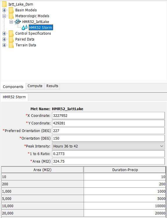
As shown in Figure 1, the HEC-HMS meteorology model’s precipitation method needs to set as HMR 52 storm and its parameters can come from the initial PMS by HEC-MetVue – see Figure 11, 12, and 13 of the first post here. The storm center X, Y coordinates are converted from longitude and latitude of PMS using NOAA NGS Coordinate Conversion Tool (NCAT). The Depth-Area-Duration data sets are paired data which also comes from the initial PMS by HEC-MetVue (Figure 2). The HMR 52 storm in HEC-HMS is a 72-hour “nested” storm in which the maximum precipitation depths of various shorter duration storms are embedded (1hr, 6hr, 12h, 24hr, 48hr).

The initial PMS of HEC-MetVue is created aiming at maximizing the precipitation depth over a basin. A PMS with the maximum precipitation depth does not necessarily generate a PMF since the runoff of a basin is not in a linear relationship with the precipitation. For this reason, the HMR 52 storm parameters in Figure 1 will need to be optimized, which can be accomplished by using HEC-HMS built-in Optimization Trial Manager (Figure 3 and 4). The optimization objective is set as peak discharge in Figure 4 and it can be changed to volume, or a stage if a reservoir element is present in the model, depending on the project needs.

All the five parameters of a HMR 52 storm can be optimized as shown in Figure 5, including X, Y coordinates, storm area, orientation, and peak intensity period. From past project experience, if X, Y coordinates are the first two parameters (Parameter 1 and 2) in an optimization trial, the optimization process may go unstable or the objective function is going to have a difficult time to converge; for this reason, X, Y coordinates may better be set as parameter 4 and 5, or they can be left out for optimization since the final result usually is insensitive to X, Y coordinates coming from HEC-MetVue HMR 52 procedures. Also, since the initial parameters entered in HMR 52 storm are from HEC-MetVue and normally they are close to the final optimized values, the parameter can use a relatively small optimization range (Minimum to Maximum) to expedite the process and avoid the optimization trial run becoming unstable.

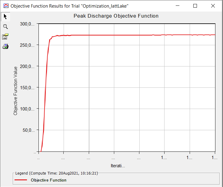
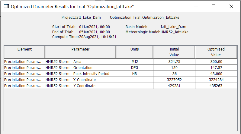
In an HMR52 storm optimization trial run, the HMR 52 storm parameters will be optimized to certain values (Figure 6) while the objective is achieving its maximum (Figure 7).

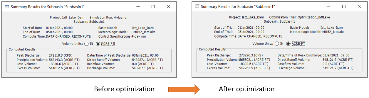
The optimization results of the parameters are shown in Figure 8 and the peak discharge comparison is shown in Figure 9 (before and after optimization). For the example model, the peak discharge is only increased by 0.44% after optimization.