Malcom Small Watershed Hydrograph Method and Its Application in Detention Design

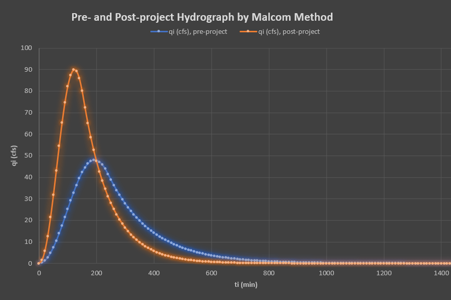
A simple hydrograph development technique, developed by H. Rooney Malcom in 1980, is often used to design detention facilities serving relatively small watersheds (less than 640 acre or 1.0 sq mi). Two hydrographs are to be developed using the Malcom Hydrograph Method for pre- and post-project conditions and the required detention volume is equal to the shaded area between the two hydrographs (Figure 1).

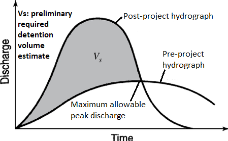
It should be noted that the final detention volume is tied to the actual basin outflow rate – if the actual basin outflow rate is much lower than the Pre-project peak discharge, the corresponding detention volume needs to be larger than the shaded area in Figure 1. For this reason, when designing a detention pond using a fixed detention rate method or Pre-/Post-project hydrograph difference method without routing the Post-project hydrograph in a H&H model, the outflow structure shall be designed in a way that its peak outflow rate matches or slightly lower than the Pre-project peak discharge.

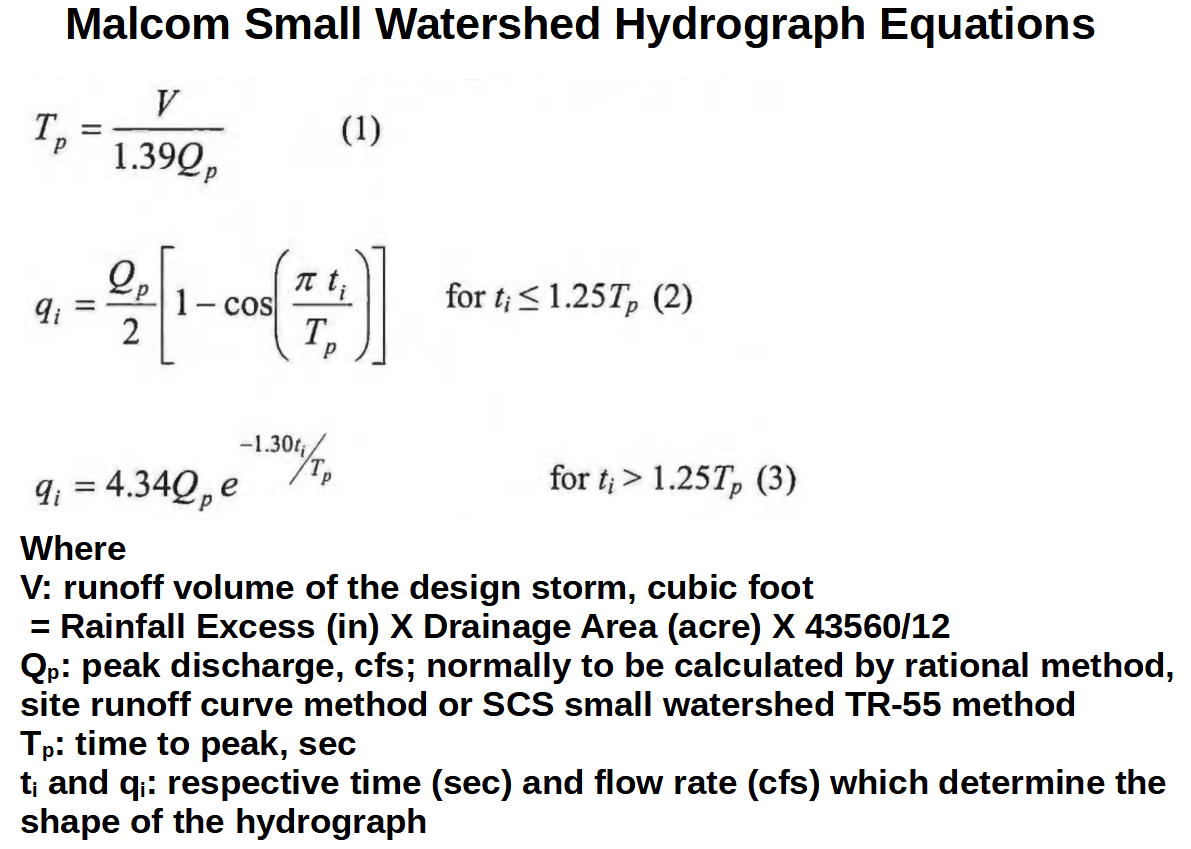
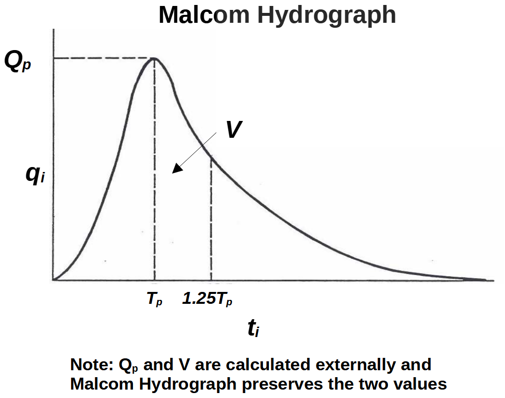
Once a small watershed peak discharge and runoff volume under a design storm are determined, Malcom Small Watershed Hydrograph Method provides a set of equations (Figure 2) to develop a runoff hydrograph which preserves the originally calculated peak discharge and runoff volume (Figure 3).

The small watershed peak discharge Qp should be calculated using methods approved by the regulating agencies such as Rational method, SCS Graphical Peak Discharge Method (refer to this Post), or Site Runoff Curve method (Harris County, TX).

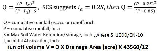
The runoff volume V of the design storm is the product of rainfall excess (direct runoff) and drainage area. SCS curve number method can be utilized to calculated rainfall excess (direct runoff) as explained in Figure 4. In practice, a 24-hr storm is usually selected as the design storm and therefore the rainfall depth P is the 24-hr precipitation depth of the selected design storm (100-yr, 50-yr, 25-yr, or 10-yr, 5-yr, 2-yr).

Harris County Flood Control District (HCFCD) recommends a set of direct runoff values (inch) of 24-hr storms for different return periods (frequencies) and impervious area conditions for runoff volume calculation (HCFCD PCPM Section 3.6).

The Malcom Small Watershed Hydrograph Method does not need a specific rainfall distribution (hyetograph) except the runoff volume (rainfall excess) of the design storm, and for this reason, it shall not be used in conjunction with other types of hydrographs including those generated from watershed HEC-HMS models or FEMA Flood Insurance Study. The time to peak of the Malcom Small Watershed Hydrograph Method is computed to match runoff volume and has no correlation with the rainfall durations and distributions used in other studies.

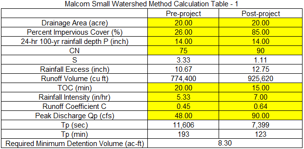
An example of Malcom Small Watershed Hydrograph Method is illustrated below for pre- and post-project conditions by using Rational Method for peak discharges and SCS curve number method for runoff volume.

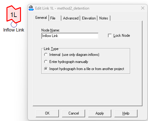
In this example, HydroCAD is used to design a detention pond using Small Watershed Hydrograph method. A post-project small watershed hydrograph time series can be saved in a CSV file which will then be imported by a Link node in HydroCAD (Figure 6 and Figure 7).

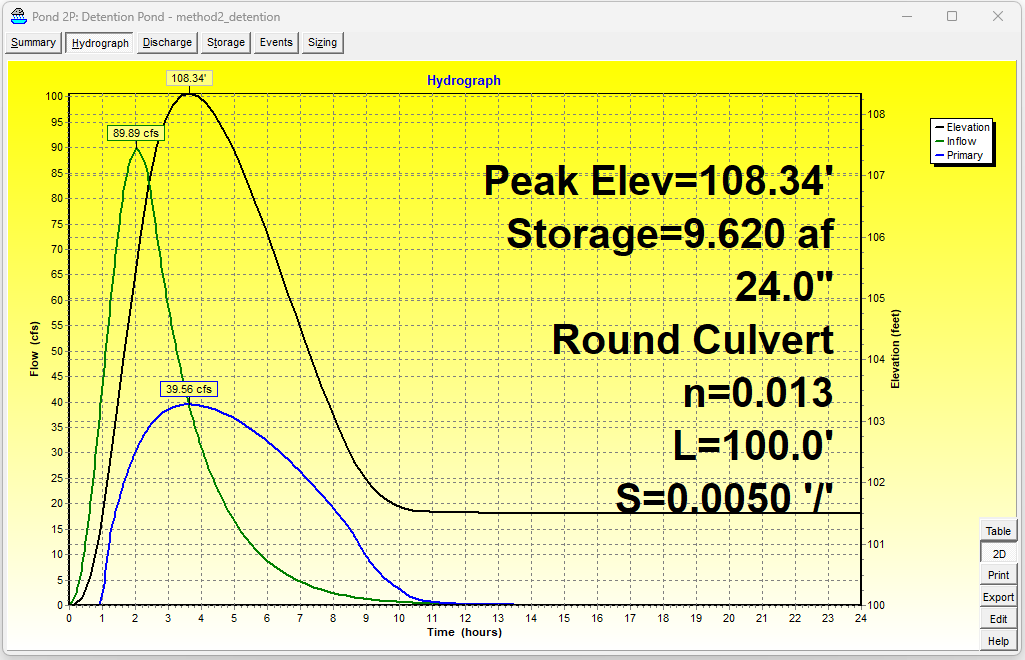
A detention pond is added to the HydroCAD model at the downstream end of the Inflow Link (Figure 8) with its routing method being Stor-Ind. The detention pond has a square shaped bottom of 190′ X 190′ at Elev 100.00′ (invert). The tailwater is set as Fixed Elevation at top of the culvert pipe (99.5+2=101.5′)

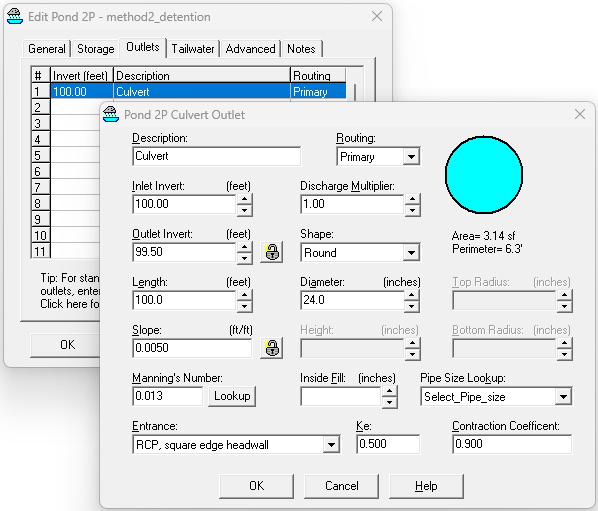
In this example, the outlet structure of the detention pond is a culvert and its size (24″ RCP, Figure 9) is finalize by trial and error method so the outflow rate is no larger than the pre-project condition (Figure 10). The example HydroCAD model can be downloaded here.

For more details about HydroCAD detention pond design, refer to Post 1 and 2.

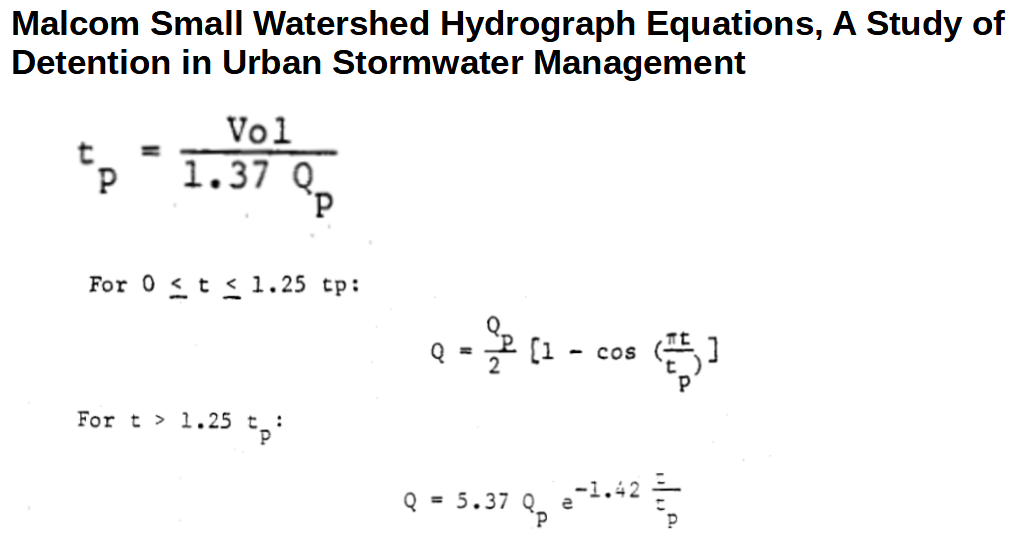
In the 1980 paper by H. Rooney Malcom, A Study of Detention in Urban Stormwater Management, the equations are somehow different as shown in Figure 11. It is unknown how the equations have evolved into today’s format.