Bridge Modeling in HEC-RAS 2D – Simplified 1D Rating Curves Approach

This article was revised and reposted because since HEC-RAS 6.7 (and the subsequent version 7.0), 2D bridge modeling has evolved significantly. The software now offers two distinct methods for simulating bridges within a 2D Flow Area. The primary difference lies in whether the bridge hydraulics are solved using pre-calculated 1D rating curves (Simplified Bridge Modeling), or a fully 2D physics-based “cloned mesh” approach (2D Pressure/Overtopping) relying on refined 2D meshes and a high resolution terrain which incorporates bridge piers and abutment geometries to resolve the details of the bridge hydraulics. This post is about the simplified bridge modeling approach and another post introduces the detailed bridge modeling methods- 2D Pressure/Overtopping.

Just like in 1D bridge modeling, a bridge can be modeled in 2D domains using a geometry editor similar to 1D bridge geometry editor. A family of bridge rating curves will be pre-calculated by HEC-RAS to account for the energy losses when water flowing through the bridge for different tailwater elevations and flows. Meanwhile, internally HEC-RAS 2D equation is going to be “tweaked” so its solution matches the energy losses over the bridge (thus also matches bridge US headwater at XS 3).

It is should be noted that the 1D rating curves bridge modeling method does not provide accurate velocity results in 2D domain since the 2D cells under the bridge do not “see” the piers or other bridge structure details. A quick way to improve the velocity result accuracy is to “burn” bridge piers and/or abutments into the underlying terrain using the terrain modification tools in addition to “build” them in the bridge geometry editor. This process will NOT “double dip” the piers effect and only generate more representative velocity results.

This post is a guidance on how to model a bridge structure in HEC-RAS 2D domain using the 1D rating curves method. You should have a working HEC-RAS 2D model before adding a bridge into a 2D domain.

1. In the main HEC-RAS Geometric Data editing window, add a SA/2D Area Connection into 2D domain (Figure 1A). The 2D connection line should be added by first clicking left end point and then working towards right when facing the downstream flow direction. The begin and end points for this 2D connection line shall be placed at bridge abutment locations to only model bridge openings, although they can be located further away from abutments.

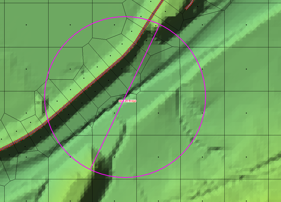
If the 2D connection line goes beyond the abutments and thus part of the roadway approaches is included as part of the bridge, then the bridge ineffective flow regions would need to be entered for the two cross sections upstream and downstream of the bridge (US Bounding XS 3and DS Bounding XS 2) by clicking Options —> Bridge Ineffective Regions… (Figure 1B).

Unless there are other valid reasons to include roadway approaches by a bridge 2D connection line, such as changing top elevations of roadway approaches by bridge deck data editor, it is recommended to model bridge openings only from abutment to abutment in a RAS 2D domain.

2. Right Click the newly added 2D connection line and select Edit Connection… to open Connection Data Editor. In Connection Data Editor, select Bridge with 1D Rating Curves for Structure Type (Figure 2).

3. Click Deck/Roadway Data Editor to type in bridge deck and roadway data. This is similar to 1D bridge data editor (Figure 3).

4. Similar to 1D bridge data editor, enter data for bridge pier, abutment, bridge modeling approach, and Htab Param. For Htab Param., head water maximum elevation and maximum flow should be provided so the 1D rating curves have enough resolution to cover the flows and elevations to be modeled.
5. In HEC-RAS 7.0 Bridge Modeling Approach, a new momentum equation called General (recommended) is introduced to replace the old one (Prismatic Legacy) for low flow bridge methods. This new momentum equation is able to provide smoother 1D rating curves. It is suggested to check on both Energy and Momentum methods for low flow condition (whichever is higher) and Pressure and/Weir method for high flow if the bridge deck is a big blockage to water flow.
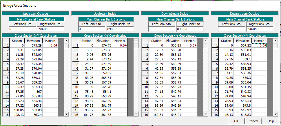
6. In Connection Data Editor, click top menu of Options and then select External and Internal Bridge Cross Sections… to enter Manning’s n value or edit the four bridge cross section data if necessary (Figure 4). Other bridge modeling options, like ineffective flow areas settings, can be edited also by go to the top menu of Options of Connection Data Editor and choose corresponding sub-menu items.

In Connection Data Editor, you can view the two bounding bridge cross sections, the two inside cross sections, and centerline over 2D faces by clicking the appropriate options of Plot (Figure 5).

7. Close Connection Data Editor and return to main Geometric Data editing window to view the bridge in 2D domain. Right click the bridge in 2D domain, select Edit Internal Connection (Break Line) Cell Spacing… (Figure 6), and type in spacing for areas around bridge break line and then enforce it by clicking Enforce Internal Connection as Break Line in 2D Flow Area (Figure 7).

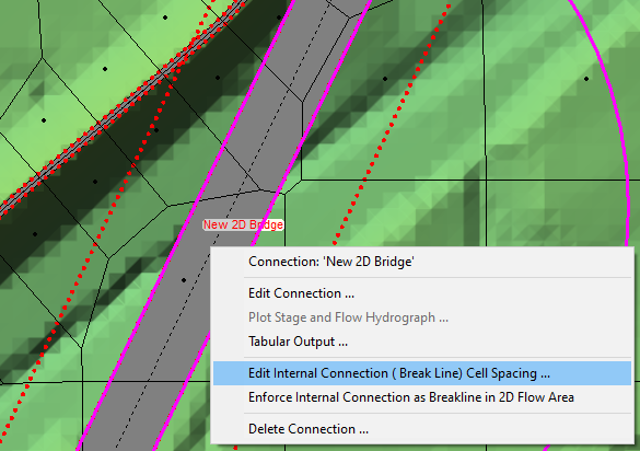
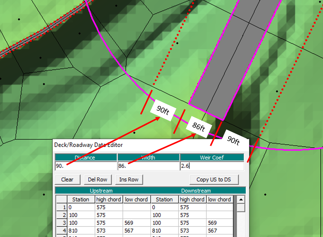
8. In Figure 6, the two red color dotted lines on each side of the bridge structure are the two bridge bounding cross section locations (cross section 3 & 2 in 1D bridge modeling) which are defined in the Deck/Roadway Data Editor (Figure 7). As in 1D bridge modeling, these two bounding cross sections represent the natural ground of the channel and overbank area just upstream and downstream of the road embankment and they are normally placed near the toe of the road embankment at each side.

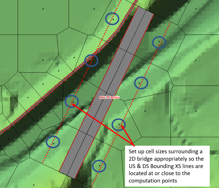
9. It is suggested that the cell sizes surrounding the bridge should be set up appropriately so the US & DS Bounding XS lines are located at or close to the computation points as shown in Figure 8.

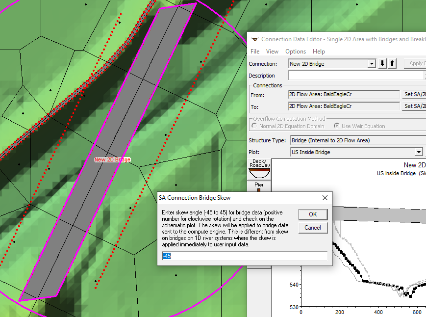
10. The HEC-RAS 1D bridge solver is used to solve bridge hydraulics in 2D domains and therefore if a bridge is skewed to the river centerline, a bridge skew angle should be provided to properly account for the bridge hydraulic opening area. For this example bridge, a negative 45 degree skew angle is entered (Figure 9).

“Burning” bridge piers into the terrain is done by using the terrain modification tool. Once the terrain is modified, the 2D meshing around the bridge piers shall be carefully adjusted by using breaklines and/or refinement regions to ensure the piers intersects with the cell faces (Figure 10).

Limitations of the simplified 2D bridge modeling approach include:

1. The velocity at or near the bridge location is not accurate;
2. The velocity particle tracing view map will show flows inside the bridge piers unless the piers are “burned” into the terrain;
3. The method is only applicable to the subcritical flow condition at a bridge location; for the supercritical flow condition, model the bridge using detailed terrain by incorporating piers and abutments in the terrain; or for supercritical high flow scenario, use the detailed 2D bridge modeling approach – the 2D Pressure/Overtopping method.