Time of Concentration (TOC) Estimation
Time of Concentration (TOC or Tc), one of the most important hydrologic parameters for runoff calculation and modeling, is defined as the time it takes a drop of rainfall to travel from the most hydraulically remote point of the drainage basin to its outlet or point of analysis. Although usually the most hydraulically remote point is located at the drainage basin divide, it is not necessarily the point having the longest distance to the outlet. After rainfall begins, the entire drainage basin starts to contribute flows at the outlet at Time of Concentration.
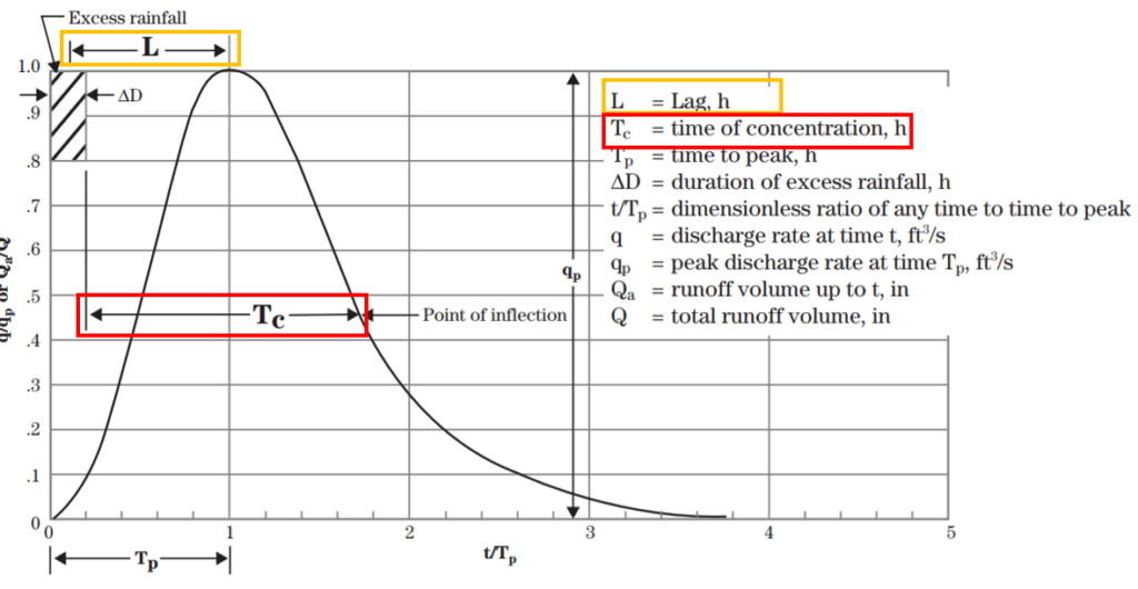
There are many factors influencing TOC, including but not limited to drainage basin area & shape, terrain, land use & urbanization, soils, natural channels and man-made drainage systems, storage effect from wetland/pond/reservoir. Usually TOC is calculated once and then the calculated values will be applied to storm events of different frequencies, even though strictly speaking TOC does vary between different storms. In hydrograph analysis, TOC can be interpreted as the time from the end of excess rainfall to the point on the falling limb of the dimensionless unit hydrograph (point of inflection) where the recession curve begins (Figure 1).
Unlike a natural drainage basin, for a man-made drainage system (example: a neighborhood or roadway storm sewer network), TOC has two basic parts, namely inlet time and flow time in storm sewer:
- Inlet time: runoff flows from the remotest point to the inlet location. The areas contributing to most storm sewer inlets are small and correspondingly the inlet time is short. Inlet time can be estimated using overland/sheet flow travel time plus shallow concentrated flow travel time. It will be rare for a channel flow to get involved to calculate inlet time.
- Flow time: water flows in storm sewer, can be calculated via Manning’s equation by assuming pipe-full flow condition – refer to the examples below.
Lag, or Lag Time, another important hydrologic parameter for unit hydrograph development, is the delay between the time runoff from a rainfall event over a watershed begins until runoff reaches its maximum peak. In hydrograph analysis, lag is the time interval between the center of mass of the excess rainfall and the peak runoff rate (Figure 1).
According to NRCS NEH Part 630 Hydrology Chapter 15, for average natural watershed conditions Lag can be estimated from TOC by the relationship of Lag = 0.6 x TOC. TxDOT Research Report 0-4696-2 proposed another relationship for watersheds in Texas: Lag = 0.4 x TOC for developed watersheds and Lag = 0.7 x TOC for underdeveloped watersheds.
There are a lot of methods to calculate TOC or Lag Time and this post only summarizes the widely recognized ones. TOC estimation is often subjective and depends greatly on engineering judgment. TOC calculation using multiple methods should always be carried out to cross-check each other’s results.
- 1. NRCS Method – perhaps the most widely used TOC estimation method
NRCS method is a velocity-based TOC method which divides a flow path into 3 or more segments and assumes TOC is the sum of travel times for each segment: TOC=T-sh+T-sc+T-ch (usually sheet flow + shallow concentrated flow + channel flow). The main drawback of NRCS method is that it requires a lot of parameters and some of them are not easy to properly estimate or acquire. Also, how to divide a flow path into different segments is often arbitrary.
1.1 Sheet flow travel time T-sh:
The sheet flow (or overland flow) happens at the beginning of a flow path where usually the depth of flow is less than 0.1 ft. The sheet flow travel time can be estimated via the equation in Figure 1A where the sheet flow length L should not be exceed 100ft. One way to estimate the sheet flow length L is to apply McCuen-Spiess equation as shown in Figure 1B.


Note: Originally, the sheet flow travel time was calculated by the Kinematic Wave Equation (Figure 1C), which requires an iterative process to solve since the rainfall intensity i depends on Tsh. This is not convenient and therefore this equation is replaced by the one in Figure 1A.

1.2 After sheet flow, shallow concentrated flow happens in swales, small rills, and gullies with a flow depth of 0.1 to 0.5ft where there is not a well-defined channel. The shallow concentrated flow length usually is less than 1000ft per TxDOT Report 0-4696-1 from engineering experience. Shallow concentrated flow travel time T-sc is calculated as:


1.3 Channel flow can be assumed to begin where either the blue stream shows on U.S. Geological Survey (USGS) quadrangle sheets or the channel is visible on aerial photographs. The velocity should be computed for normal depth (uniform flow condition) based on bank-full flow conditions. Flow with return periods from 1.5 to 3 years (2-year as the average) is often assumed to produce bank-full condition.

When applying NRCS method, if a flow segment is not present for a specific drainage area, its travel time will be zero. On the other hand, sometimes it may be more appropriate to further divide the entire flow path into more than three segments to better describe flow characteristics along the path, for example, in addition to open channel segment, another flow segment may need to be defined if part of the flow path is a storm sewer system. In the example TOC calculation in Figure 5, there is no segment for open channel flow, but a new segment of storm sewer flow is added to flow path scheme to account for travel time in storm sewer system.

- 2. Kerby-Kirpich Method
Kerby-Kirpich is a popular TOC estimation method and it does not require as many parameters as NRCS method does. In Kerby-Kirpich method, TOC consists of two types of travel times: overland flow time calculated by Kerby equation and the channel flow time by Kirpich equation: TOC = T-ov+T-ch. TxDOT prefers Kerby-Kirpich method for TOC estimation since it is straightforward to apply and produces readily interpretable results.
2.1 Overland flow travel time T-ov is calculated by Kerby equation (Figure 6)


TxDOT Hydraulic Design Manual recommends an upper limit of 1200ft for the overland flow length in Kerby equation.
2.2 Channel flow travel time T-ch is calculated by Kirpich equation (Figure 7)

2.3 Slope adjustment for Kerby-Kirpich method
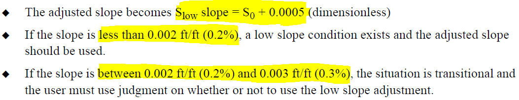
TxDOT Hydraulic Design Manual recommends that too flat a slope should be adjusted by 0.0005 to avoid an unreasonably large TOC value (Figure 8) from Kerby or Kirpich equations.
An example to calculate TOC for a roadway drainage area is illustrated in Figure 9. In this example, the last segment of flow is within a storm sewer pipe, Kirpich method equation is not appropriate. Instead, the travel time is calculated by velocity from Manning’s Equation.

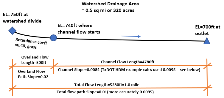
TxDOT HDM gives another example of Kerby-Kirpich method for a small watershed of 0.5 square mile in Chapter 4 (Figure 10). The overland flow travel time by Kerby equation is about 25 minutes and the channel flow travel time is 34min (32min if channel slope is taken as 0.0095). The total TOC is 59min.
In the book of Applied Hydrology, Ven Te Chow suggested that TOC calculated from Kirpich method be adjusted by multiplying 0.4 for concrete/asphalt surface overland flow and 0.2 for flow in concrete channels. Although TxDOT Hydraulic Design Manual does not recommend such an adjustment, it is prudent to pay special attention to TOC results whenever applying Kirpich method over asphalt or concrete surface/channel.
- 3. Average velocity Method
Another simple but quite useful velocity-based TOC method is the average velocity method per Harris County Flood Control District POLICY, CRITERIA, AND PROCEDURE MANUAL (HCFCD PCPM). Similar to NRCS method, the flow path is divided into different segments: overland flow, gutter flow, roadside ditch flow, storm sewer flow, channel or ditch flow, and the total TOC is the sum of each segment travel time: TOC= T-1+T-2+…+T-n. For each segment travel time T-i, only two parameters are needed: segment flow path length L (ft) and the average flow velocity V (fps) which can be looked up in Table 3 or Table 4.
T-i=L/(60*V), minutes


An example to calculate TOC for a roadway drainage area using average velocity method is illustrated in Figure 11.

Some regulating agencies requires adding additional 10 min or 15 min to the time of concentration calculated by the average velocity method, such as City of Sealy, TX and Brazoria Drainage District No. 4 (Figure 11A). According to City of Sealy Drainage Criteria Manual, the initial time of 10 minutes is added to the overall time of concentration to to account for the initial delay between the start of rainfall and development of actual surface runoff. A modeler should only account for the initial time when the regulating agencies have such a specific requirement.

- 4. FAA Method
Federal Aviation Administration developed a TOC equation in 1970 from airfield drainage data (Figure 12).
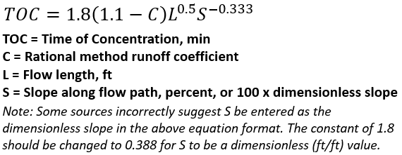
Example: C=0.9, L=1000ft, S=0.006=0.6%, TOC=1.8x(1.1-0.9)x1000^0.5×0.6^(-0.333)=13.5 minutes. In the above equation format, if S is entered as a dimensionless value of 0.006 as some other sources suggested, the TOC will be unreasonably large, 62.5 minutes.
FAA method is probably most valid for small watersheds in a urban basin where sheet flow or overland flow controls. FAA method tends to overestimate inlet time if the inlet time flow path has a significant portion of shallow concentrated flow. For the reasons above, FAA method is not recommended for TOC calculation unless overland flow overwhelmingly dominates the entire flow path.
- 5. Drainage Area Method
City of Houston, City of Dickinson, and some other city drainage design manuals endorse the use of a simple TOC method whose only parameter is the drainage area A (Figure 13). According to City of Dickinson Drainage Criteria Manual, this method can accurately estimate TOC for sewer projects; however it tends to underestimate actual TOC for basins with significant overland flow or open ditch flow, and therefore may overestimate peak runoff flow rates for these basins. Since this method does not distinguish inlet time from flow time in storm sewer, it is reasonable to assume it just lumps them together into one TOC value.

An engineer should be very careful when applying the drainage area method to calculate TOC since a lot of regulating agencies do not approve a TOC method which is not based on velocities. It is recommended that this method should only be used for cross-checking TOC results calculated by other methods, unless a client specifically approves its use for design and modeling.
Example: Drainage Area A=120 acres, and TOC=10 x 120^0.1761+15 = 38.2 minutes.
- 6. TxDOT Drainage Area Square Root Method
TxDOT Hydraulic Design Manual introduces a TOC ad hoc method which takes the square root of a drainage area (Figure 14). It is unknown how this drainage area square root method was originally developed and therefore the method should only be used for results backchecking.
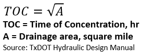
Example: Drainage Area A=0.5 square mile, and TOC=0.5^0.5 hr = 0.71hr or 42 minutes.
TxDOT Research Report 0-4696-2 includes a graph to show the relationship of TOC and drainage areas by different methods (Figure 15). Amazingly, TOC calculated from this ad hoc method passes through the generalized data point center for drainage area ranging from 0.2 to 200 square mile.

- 7. Bransby-Williams Method
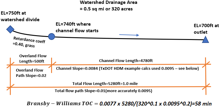
Bransby-Williams method was developed in 1920’s from spillway flood discharge studies in India (Figure 16 and Figure 17).


Bransby-Williams method is most likely appropriate for natural rural watersheds due to its origin.
Hongkong Government GEO Report No. 292 recommends the use of Bransby-Williams method for time of concentration calculation for natural terrain catchments, but where the stream course has been channelized and straightened, Bransby-Williams method tends to overestimate time of concentration: to mitigate this issue, it is suggested to calculate the travel time of channel flow separately.
For comparison, the TxDOT HDM Chapter 4 example watershed TOC was re-calculated by Bransby-Williams method as 58 min, which is surprisingly close to the value from Kerby-Kirpich method (Figure 18).
- 8. NRCS Lag Time Method
According to NEH Part 630 Hydrology, the NRCS Lag Time Method (Figure 19) is suitable for different watershed conditions ranging from heavily forested watersheds with steep channels and a high percent of the runoff resulting from subsurface flow, to meadows providing a high retardance to surface runoff, to smooth land surfaces and large paved areas. The curve number CN used in the equations should NOT be less than 50, or greater than 95.
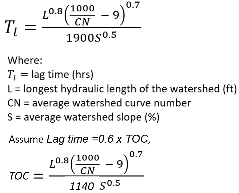
The NRCS Lag Time Method was developed using data from 24 watersheds ranging in size from 1.3 acres to 9.2 square miles by Mockus in 1961. Folmar and Miller revisited the development of this equation using additional watershed data and found that a reasonable watershed area upper limit may be 19 square miles.
There are other methods for TOC estimation although these methods are not popular or easy to use. TxDOT Report 0-4696-1 summarized various TOC methods and they can be reviewed here.
Some thoughts on which TOC method to use for a drainage design or modeling project:
- Apply whatever TOC methods designated by a client’s drainage design criteria and manuals
- Select a TOC method you feel comfortable with, such as a velocity-based TOC method or Kerby-Kirpich method, if a client has no preference
- Use a different TOC method to evaluate TOC results to gain confidence
- Verify the calculated TOC is no less than the required minimum TOC, and otherwise use the minimum TOC instead of the small calculated values. Example: Min. of TOC=10min for TxDOT projects; UDFCD (now rebranded as MHFD) requires a minimum TOC of 5 minutes for urbanized areas and 10 minutes for areas not considered urban.
- Re-calculate TOC, if possible and warranted, through model calibration
- It seems prudent to always verify TOC by using the average velocity method which is simple and straightforward.
Flow path slope calculation
A lot of TOC methods require the calculation of slopes along flow paths. A simple and straightforward way is to calculate an average slopes by considering the most upstream and downstream elevations along the flow path (Figure 20). However, this slope sometimes is not representative and it is often being distorted by a steep upper portion of a watershed or a highly irregular profile. To correct this issue, the 10-85 slope can be used for a better representation of an overall flow path as illustrated in Figure 20.

1 COMMENT