Watershed Delineation Using TauDEM Plugin in QGIS
TauDEM, developed by Utah State University is a set of tools to extract and analyze hydrologic information from topography as represented by a DEM. TauDEM is a set of standalone command line executable programs, but can also be installed in ArcGIS as a toolbox or in QGIS as a Plugin for easy application. Refer to this post on how to install TauDEM Plugin in QGIS.
To delineate a watershed upstream of an outlet (point of analysis), several steps are generally required:
- Acquire a DEM of the area of interest and re-project it to a projected coordinate system, if it is in a geographic coordinate system originally;
- Remove pit/fill sink;
- Calculate flow direction;
- Calculate flow accumulation and stream network;
- Specify an outlet location which is the point of analysis;
- Delineate watershed upstream of the outlet specified.
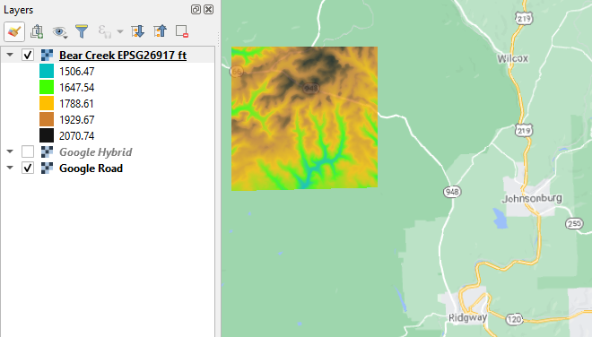
This post demonstrates the watershed delineation method using TauDEM Plugin in QGIS. This demonstration is for Bear Creek watershed, located at about 9 miles west of Johnsonburg, PA (Figure 1). DEM is downloaded from USGS National Map and a step by step instruction of downloading USGS DEM can be found in this post. USGS DEM’s CRS is in EPSG 4269 with elevation unit in meter. Prior to commencing watershed delineation, the USGS DEM was re-projected to UTM Zone 17N (EPSG 26917, NAD83) and clipped to an area just bigger than supposed watershed to reduce DEM file size. The DEM elevation was converted to foot using QGIS raster calculator.
The files used for this demonstration can be downloaded here including the re-projected DEM file Bear Creek EPSG26917 ft.tif, outlet shapefile, the final delineated watershed shapefile, and Bear Creek watershed shapefile of HUC12 050100050603.
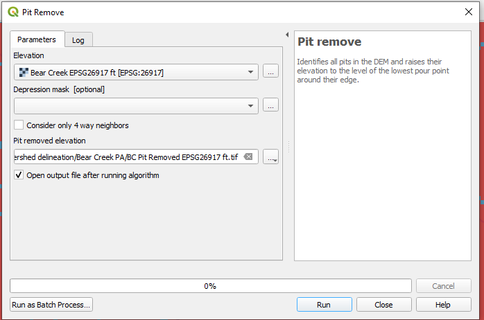
- Pit remove (Figure 2): the input file is the re-projected DEM file – Bear Creek EPSG26917 ft.tif and the output file is a new hydraulically connected DEM – BC Pit Removed EPSG26917 ft.tif.
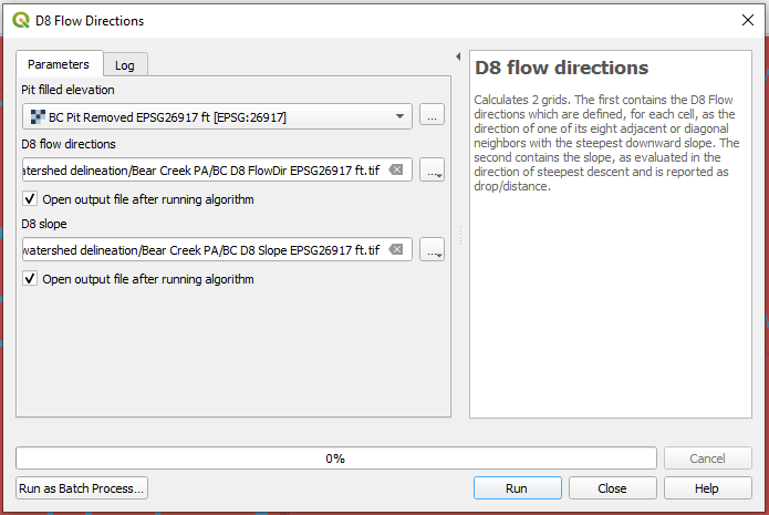
- Run D8 Flow Directions (Figure 3): the input file is the new hydraulically connected DEM – BC Pit Removed EPSG26917 ft.tif and the output files are D8 Flow Directions file – BC D8 FlowDir EPSG26917 ft.tif and D8 Slope file – BC D8 Slope EPSG26917 ft.tif.
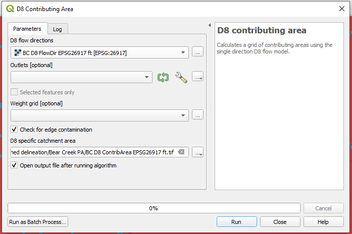
- Run D8 Contributing Area (Figure 4): the input file is the D8 Flow Directions file – BC D8 FlowDir EPSG26917 ft.tif and the output file is BC D8 ContribArea EPSG26917 ft.tif. At this step, Outlets [optional] is left as blank and it is recommended to check on “Check for edge contamination“.
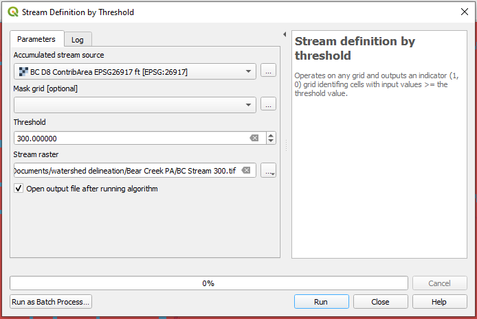
- Run Stream Definition by Threshold (Figure 5): the input file is the D8 Contributing Area file – BC D8 ContribArea EPSG26917 ft.tif and the output file is BC Stream 300.tif. At this step, Mask grid [optional] is left as blank and the threshold value is settled at 300 after trial & error. A smaller threshold value will result in a denser stream network.
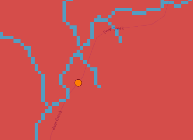
- Create a point shapefile with a single point as the outlet location using QGIS (the yellow point on Figure 6). The outlet location will be your point of analysis. Ideally this point should be located on the stream network defined at Step 4 (blue pixels on Figure 6), however it is difficult or sometimes impossible to put this point on stream network at first attempt. This is acceptable: in this example, as shown on Figure 6, the outlet is located on the Bear Creek stream line of the background google map, not on the blue pixels. At next step, this point will be slightly relocated to the blue pixels (stream network) using Move Outlets to Streams of TauDEM.
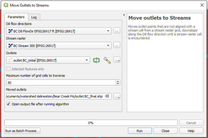
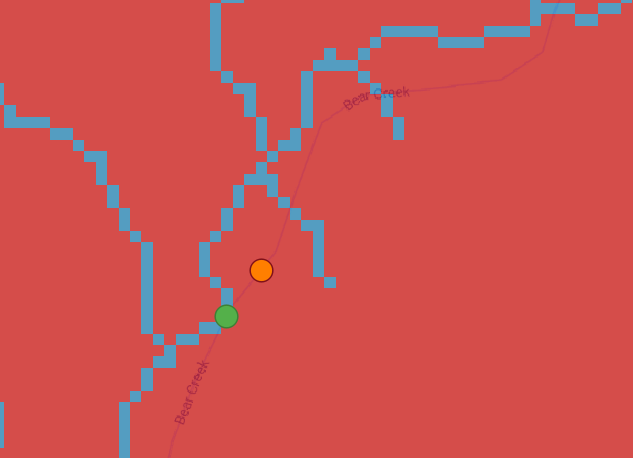
- Run Move Outlets to Streams (Figure 7 and Figure 8): Input files are D8 flow directions file from Step 2, Stream raster file from Step 4, and initial outlet point shape file from Step 5. The output file is the relocated outlet point shapefile of outlet BC_final.shp. As shown on Figure 8, the relocated outlet is located exactly on the stream network (green point on blue pixels).
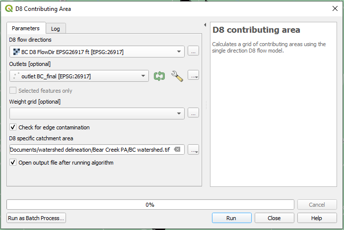
- Run D8 Contributing Area gain (Figure 9): After the final outlet point shapefile is created at Step 6, run D8 Contributing Area again to delineate the watershed (upstream area) of the outlet. Different from Step 3, here Outlets [optional] is selected as outlet BC_final.shp from Step 6. It is recommended to check on “Check for edge contamination”. The output file of this step is BC watershed.tif.
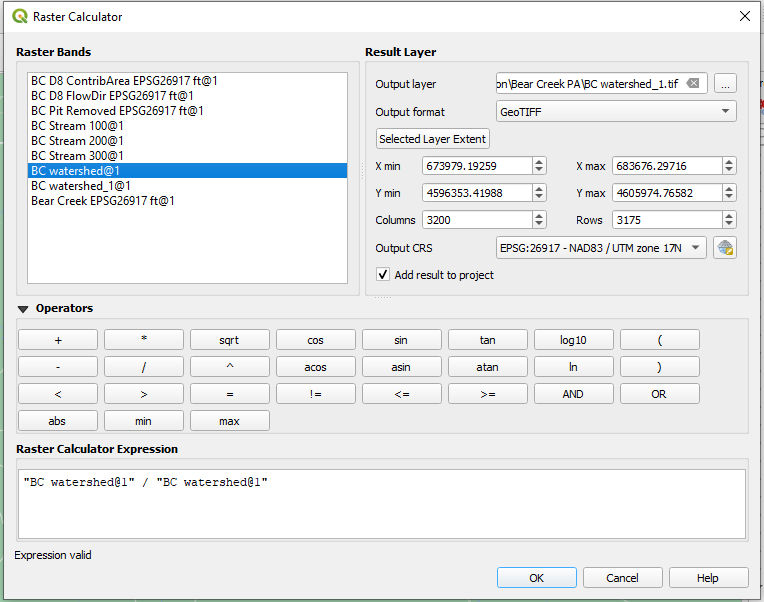
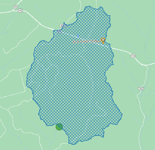
- Convert the output raster file of Step 7 (BC watershed.tif) to a raster file with a homogeneous cell value of 1 using QGIS raster calculator (BC watershed_1.tif, Figure 10 and Figure 11). A lot of GIS hydrology spatial analysis tools require that a watershed raster file has a single cell value. The output file of this step is a new watershed raster file with single cell value of 1 – BC watershed_1.tif.
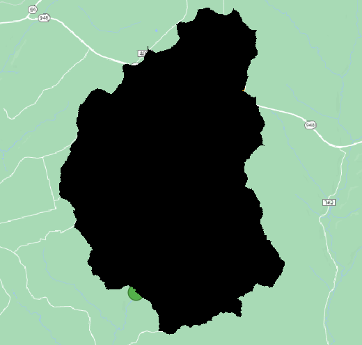
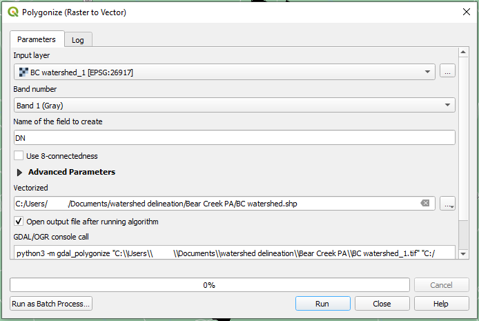
- Vectorize the output raster file of Step 8 (BC watershed_1.tif, Figure 12 and Figure 13). The final watershed shapefile is BC watershed.shp
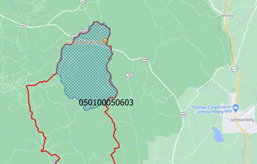
Finally to back check the watershed delineated. HUC12 050100050603 was downloaded from USGS National Map (refer to this post on how to download NHD Dataset including HUC shapefile) and superimposed over BC watershed.shp. As shown on Figure 14, the watershed delineated is the upper portion of HUC12 050100050603 and it matches well with the NHD boundary (red line).
Leave a Reply