Watershed Delineation Using Whitebox Tools (WBT) Plugin in QGIS
Whitebox Tools (WBT) is an advanced geospatial data analysis platform developed by Whitebox Geospatial, Inc. WBT contains plenty of tools to process various types of geospatial data for H&H analysis. WBT can serve as an analytical Plugin for QGIS, a free and open source GIS tool. Refer to this post on how to install Whitebox Tools (WBT) Plugin in QGIS.
To delineate a watershed upstream of an outlet (point of analysis), several steps are generally required:
- Acquire a DEM of the area of interest and re-project it to a projected coordinate system, if it is in a geographic coordinate system originally;
- Remove pit/fill sink;
- Calculate flow direction;
- Calculate flow accumulation and stream network;
- Specify an outlet location which is the point of analysis;
- Delineate watershed upstream of the outlet specified.
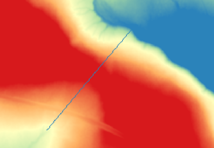
This post illustrates the watershed delineation method step by step using Whitebox Tools (WBT) Plugin in QGIS. This demonstration is for Bear Creek watershed, located at about 9 miles west of Johnsonburg, PA (Figure 1). The DEM is downloaded from USGS National Map and a step by step instruction of downloading USGS DEM can be found in this post. USGS DEM’s CRS is in EPSG 4269 with elevation unit in meter. Prior to commencing watershed delineation, the USGS DEM was re-projected to UTM Zone 17N (EPSG 26917, NAD83) and clipped to an area just bigger than the supposed watershed to reduce DEM file size. The DEM elevation was converted to foot using QGIS raster calculator.
Sometimes it is necessary to re-condition the raw DEM by carving a stream or raising a wall into it before the watershed delineation process (Figure 1). Several tools are available to do it including r.carve (Grass GIS), FillBurn (Whitebox Tools), or RaiseWalls (Whitebox Tools). Normally you need to prepare a linear shapefile first to denote the stream and the wall alignments.
- Fill Depressions (Figure 2): In this example, FillDepressionsWangAndLiu is used to fill any depressed low spots within the DEM. The input file is the re-projected (or re-conditioned) DEM and the output file is a new hydraulically connected filled DEM. In Figure 2, the option of Fix flat areas? should be checked on and Flat increment value (z units) can be left as Not set or a very small number such as 0.001.

Sometimes the operation of fill depression will have a substantial impact on the original DEM which may cause a problem to the following watershed delineation. To avoid this drawback and minimize the impact, the DEM can be first breached using BreachDepressions tool before being filled – refer to this post for details.
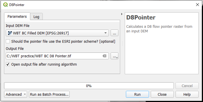
- Run D8 Pointer (Figure 3): The input file of D8Pointer is the new filled DEM – WBT BC Filled DEM.tif and the output files is WBT BC D8 Pointer.tif. Don’t use FD8Pointer at this step!
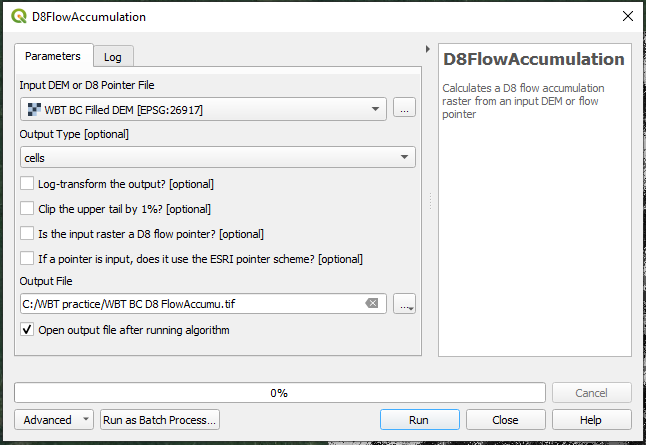
- Run D8 Flow Accumulation (Figure 4): The input file of D8FlowAccumulation is the new filled DEM – WBT BC Filled DEM.tif and the output file is WBT BC D8 FlowAccumu.tif. The Output Type is set as cells.
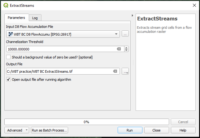
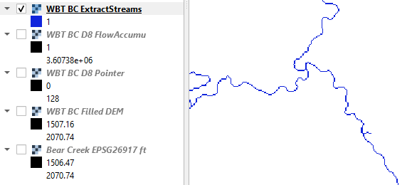
- Run Extract Streams (Figure 5): The input file of ExtractStreams the D8 Flow Accumulation file – WBT BC D8 FlowAccumu.tif and the output file is WBT BC ExtractStreams.tif. In this example, Channelization Threshold is set as 10000. This number should be settled down after trial & error. A smaller threshold value will result in a denser stream network. The extracted stream network raster file is shown in Figure 6A.
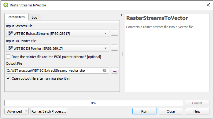
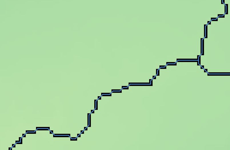
The extracted streams in raster format can be vectorized using RasterStreamsToVector tool (Figure 6B). The result is shown in Figure 6C.
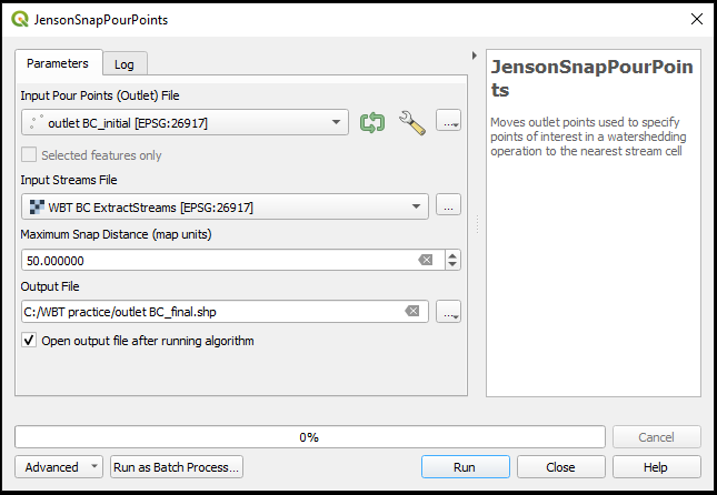
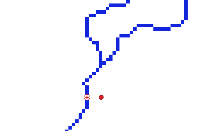
- Create a point shapefile with one or more points at the outlet locations using QGIS. The outlet locations are the points of analysis. Ideally the points should be located on the stream network defined at Step 4 (blue pixels on Figure 6), however it is difficult or sometimes impossible to put this point on stream network at first attempt. Whitebox Tools (WBT) Plugin has a function to move any initial outlet location points to the extracted stream network – JensonSnapPourPoints (similar to TauDEM Plugin’s Move Outlets to Streams). As shown in Figure 7, the Input files are the initial outlet point shapefile and the extracted stream network raster file, while the output file is another point shapefile whose points are exactly located on the streams (Figure 8). The Maximum Snap Distance is set as 50 in this example.
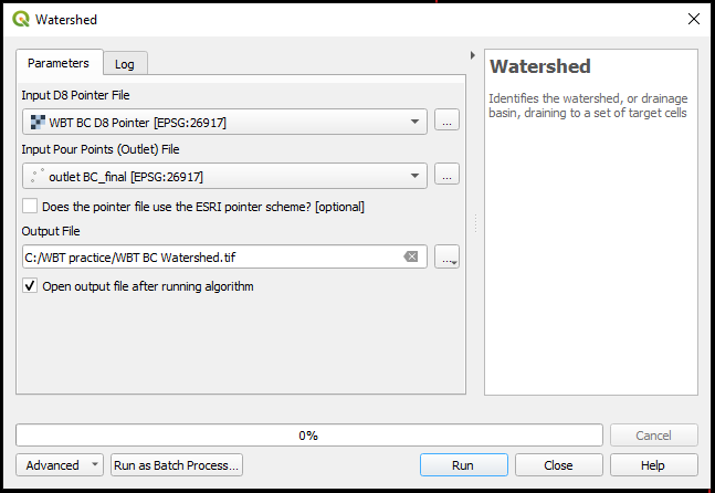
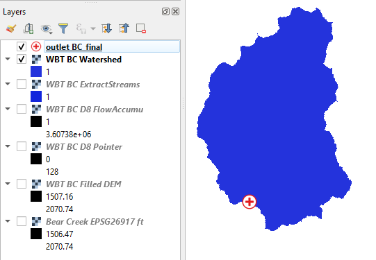
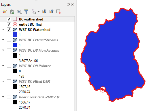
- Run Watershed delineation (Figure 9): After the final outlet point shapefile is created at Step 5, run Watershed of Whitebox Tools (WBT) to delineate the watershed (upstream area) of the outlets. The input files are the D8 Pointer file and the relocated outlet point shapefile; while the output file is a watershed raster file (Figure 10).
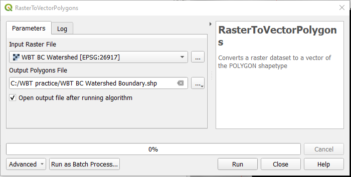
- Use RasterToVectorPolygon tool of WBT (Figure 11) to vectorize the output raster file of Step 6 if a watershed shapefile is preferred and the final watershed shapefile is shown on Figure 12.
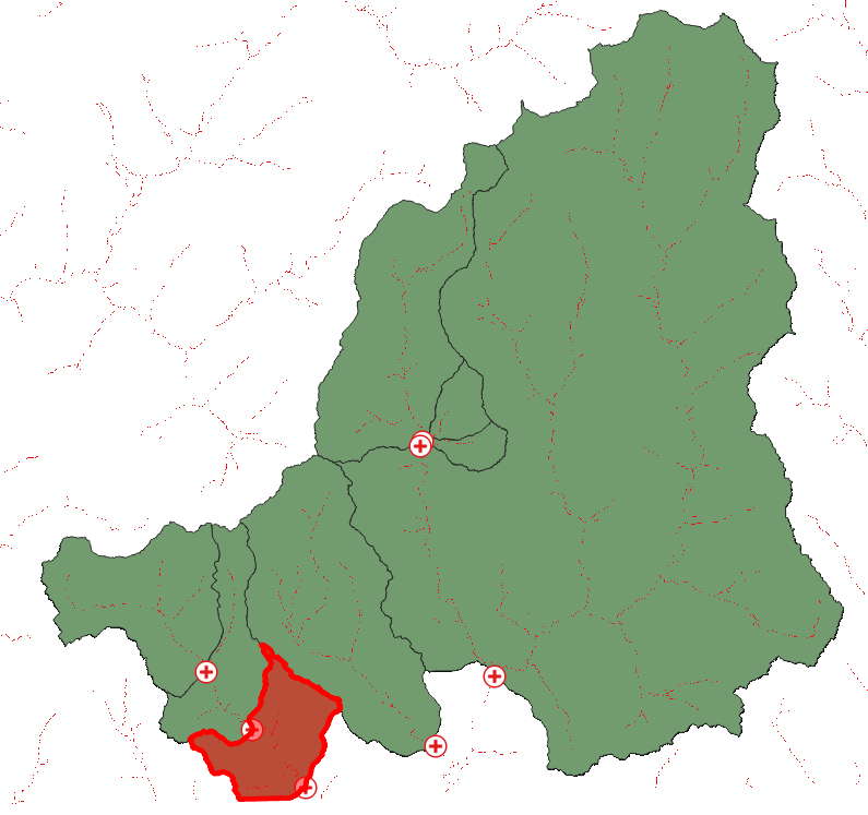
At step 6, if the outlet point shapefile contains multiple points, the resulted watershed shapefile is a watershed basin group which contains “nested” basins corresponding to each of the the outlet points (Figure 13). In a “nested” basins group, the drainage area of an outlet is only delineated up to its immediate upstream outlet point, and thus it is not a complete watershed (the red highlighted area in Figure 13).
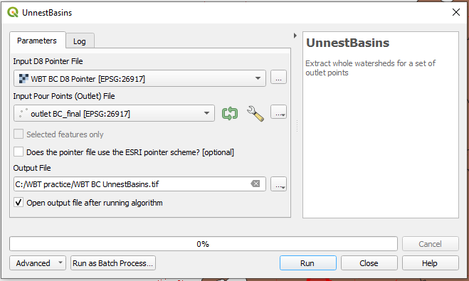
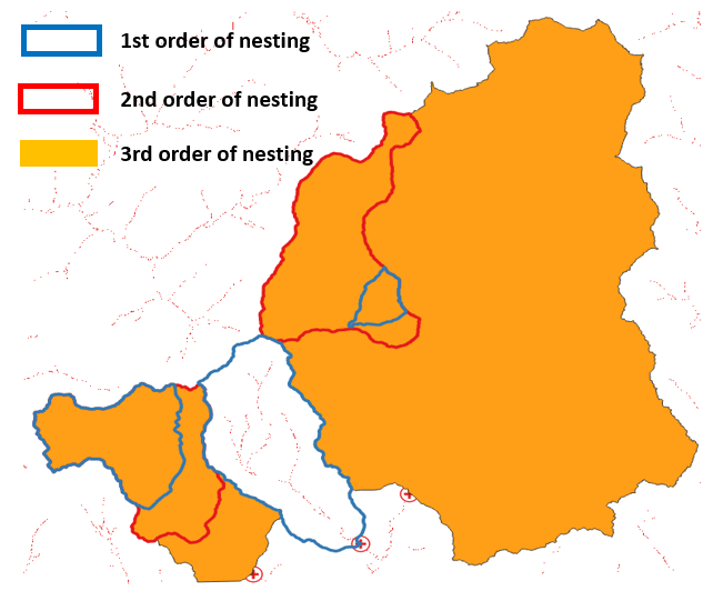
WhiteboxTools has another tool, UnnestBasins, to create a complete watershed for each of the outlet points (Figure 14). UnnestBasins shares the same input files as the Watershed tool, but its output is a series of drainage basin raster files and each of them contains one or more complete drainage basins which are on the same order of nesting. In this example, the total number of nesting order is 3, so there are 3 output files – WBT BC UnnestBasins_1.tif, WBT BC UnnestBasins_2.tif, and WBT BC UnnestBasins_3.tif and their corresponding polygon shapefiles after conversion are shown in Figure 15.
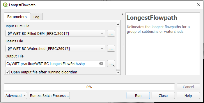
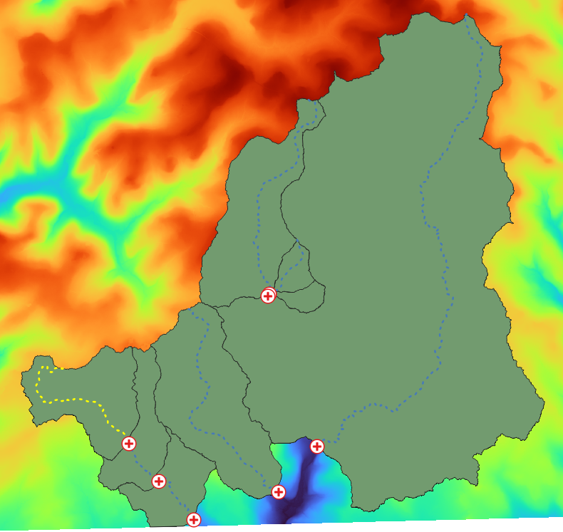
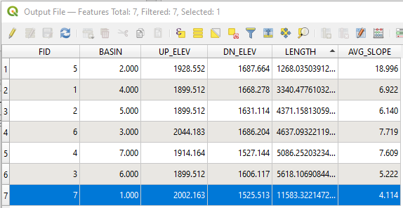
The longest flow path of a watershed can be calculated using the LongestFlowPath tool of WBT (Figure 16) and the result shapefile (Figure 17) including attribute values such as flow path lengths, upstream and downstream elevations, and slopes in percentage (Figure 18), which are often required to calculate time of concentration.
Leave a Reply