Calculate Area-Weighted Average Curve Number Using Land Cover Raster File and HSG Raster File in QGIS (1 of 3)

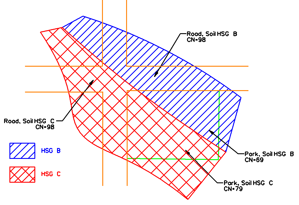
The SCS (NRCS) Curve Number is used to quantify infiltration loss during runoff calculation. As illustrated in Figure 1, the CN is determined by both soil types (Hydrologic Soil Groups, or HSG A, B, C, D) and land cover types (land use). The average CN of a watershed is the area-weighted average CN of each combination of soil type and land cover type. Note: As of 2022, there is an easier way to create a curve number raster file in RAS Mapper – refer to this post.

To use QGIS spatial analysis function to determine the overall CN, first two raster files – Land Cover Raster file and HSG Raster file need to be created and then a third raster file – CN raster file will be derived using GDAL Raster Calculator to assign CN for each combination of soil type and land cover type. Finally Zonal Statistics tool of QGIS is applied to calculate area-weighted average CN. This post (1 of 3) is to create a Land Cover Raster file and the 2nd post (2 of 3) is about how to create HSG Raster file. The 3rd post (3 of 3) is an instruction of combining Land Cover Raster file and HSG Raster file to generate a CN raster file for calculating an overall CN.

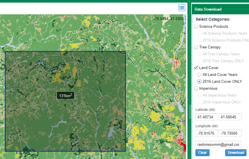
1. Go to mrlc.gov/viewer/ to download the latest NLCD raster file for your project area. Draw a big rectangular box to ensure that the project area is well covered. After providing an email address and clicking the Download button in Figure 2, click the link in the email from MRLC to download the raster files (in a zip file).

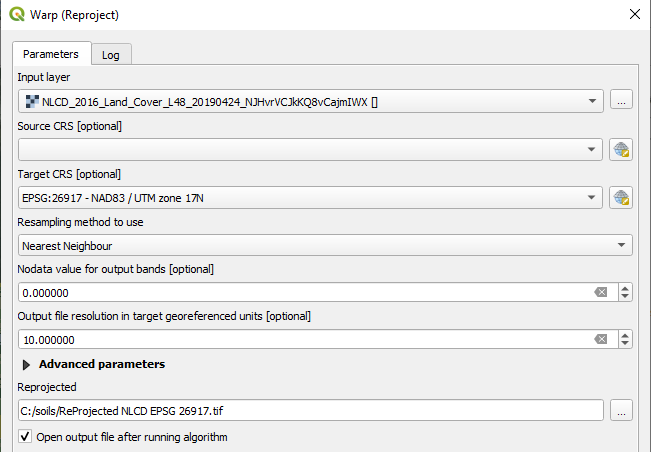
2. The download NLCD raster file is in EPSG 5070 and it needs to be re-projected to the project CRS (EPSG 26917, UTM Zone 17N for the example in Figure 3). For NLCD raster file re-projection, the Resampling method to use needs to be set as Nearest Neighbour to keep the NLCD Land Cover classification numbering system intact. In the example of Figure 3, set Nodata value for output bands as zero and Output file resolution in target georeferenced units as 10 (10 meter since EPSG 26917 Unit is meter)

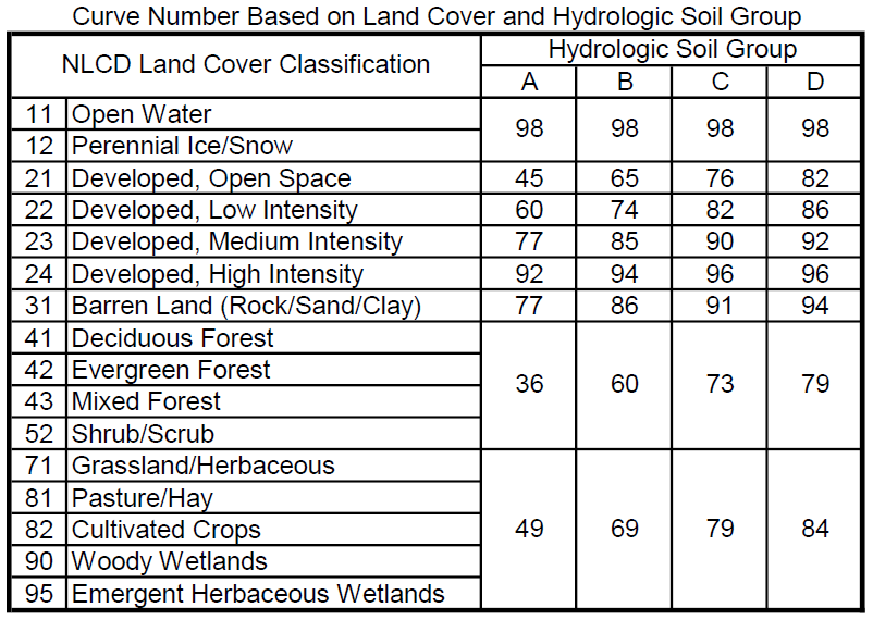
3. NLCD dataset has 20 different types of land cover types. If we leave the original land cover types alone, when combined with HSG soil types (A, B, C, D) it may end up with max. 20 x 4=80 different combinations for CN assignment. This is enormous work and sometime it is not feasible to really discretize 80 different combinations for CN assignment purpose. Utilizing NLCD raster file reclassification to reduce land cover categories is a common way to simplify and streamline CN calculation procedure.
4. It is a judgment call on how to reclassify NLCD raster file. Table 1 shows a reclassification method to reduce land cover types to 8 and CN assignments to 8 x 4=32 combinations of soil and land cover types. You are encouraged to use a different curve number table to meet your project requirements and design guidelines. Table 2 is another curve number table without reclassifying NLCD raster file.

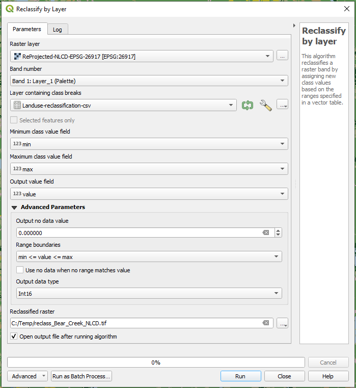
5. Use Reclassify by layer tool to reclassify the NLCD raster file (Figure 4). A CSV txt file for class breaks should be created and added to QGIS layer panel (A sample CSV class break txt file for download which is written per Table 1). on Figure 4, Output no data value is set as zero and Range boundaries is set as min<=value<=max for the sample class break txt file, but you can choose other Range boundaries method depending on your own class break txt file. The Output data type is chosen as Int16 (integer number).

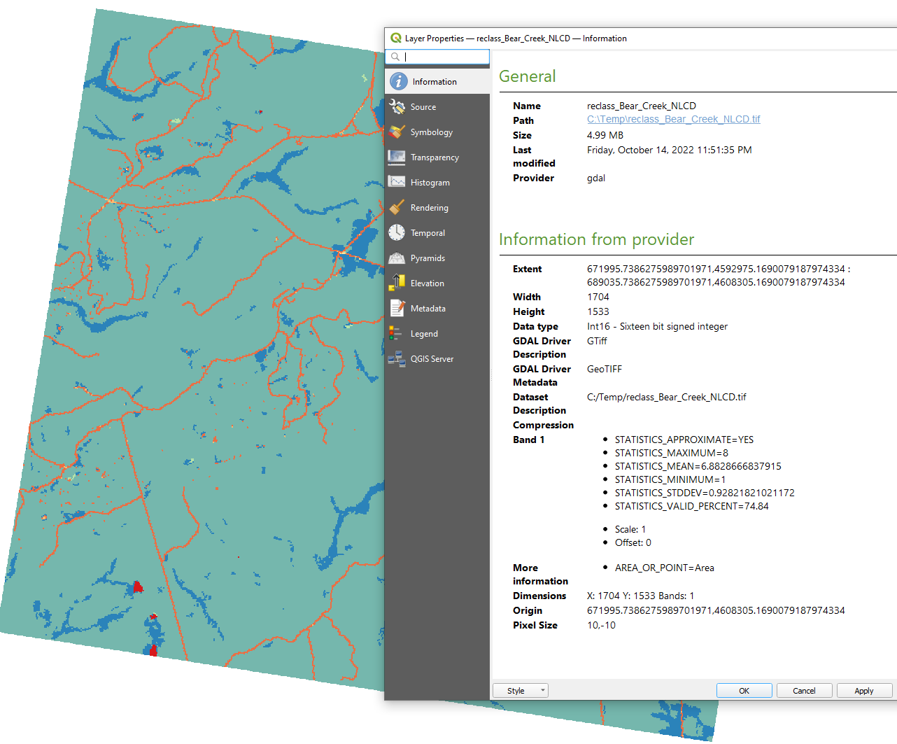
6. Check the new reclassified NLCD raster file (Figure 5) and it appears the results are correct as intended (10 meter pixel size, CRS in EPSG 26917 with meter as Unit).

Some example files used in the demonstration for downloading:

• Original NLCD raster file (EPSG 5070)
• Re-projected NLCD raster file (EPSG 26917, UTM Zone 17N)
• Sample CSV class break txt file
• Reclassified land cover raster file (EPSG 26917, UTM Zone 17N)