Create a Curve Number Raster File from Infiltration Layer in RAS Mapper

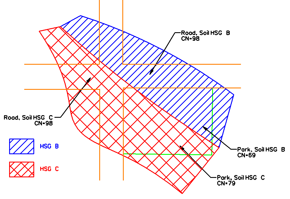
The SCS Curve Number (CN) is used to quantify infiltration loss during runoff calculation. As illustrated in Figure 1, a curve number should be determined by soil (Hydrologic Soil Groups, or HSG A, B, C, D) and land cover types (land use). A more detailed introduction about Curve Number Method and its application in HEC-HMS and InfoWorks ICM can be found here.

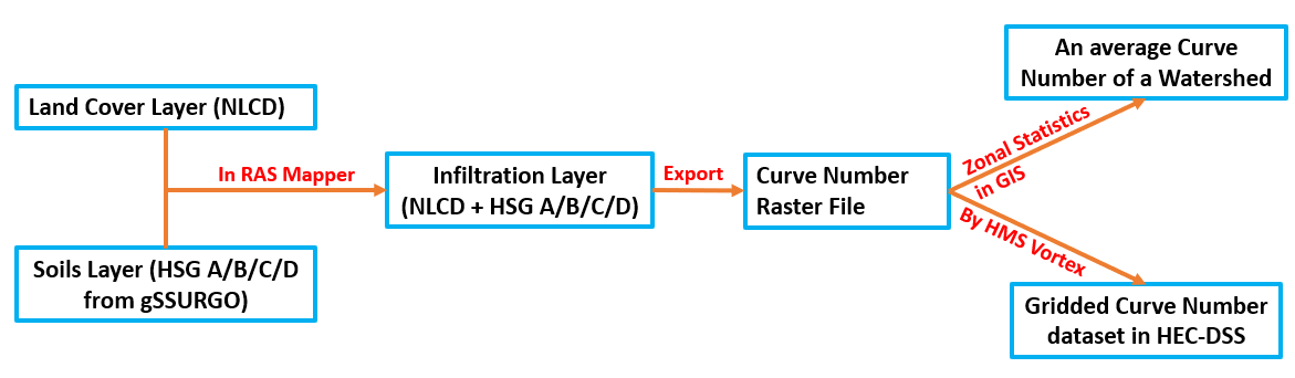
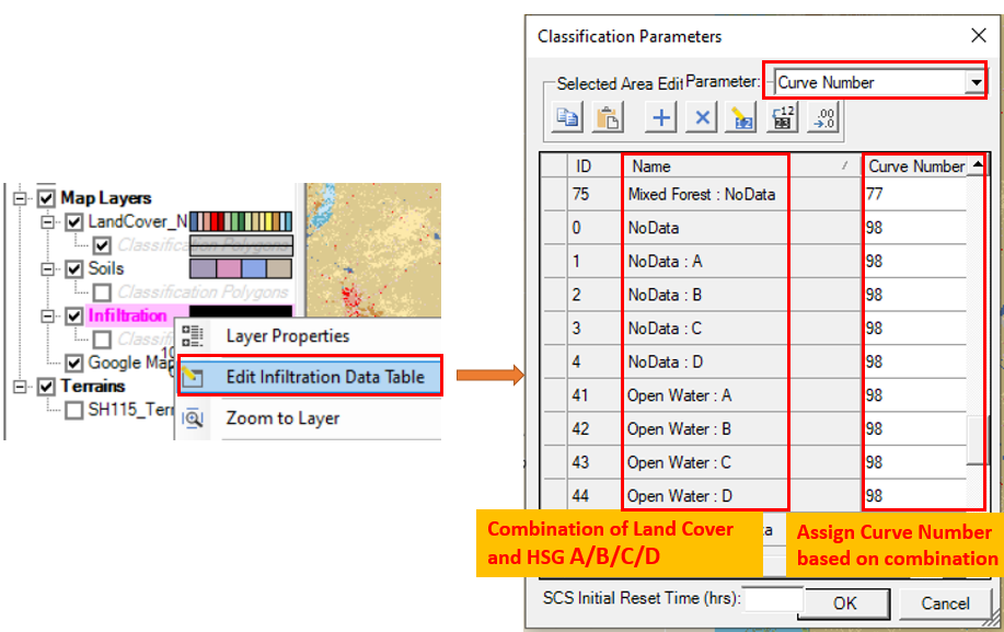
In RAS Mapper, a NLCD raster file (land cover layer) and a HSG raster file (soils layer) can be intersected through the creation of an infiltration layer in which different curve numbers will be assigned to different combinations of land cover and soil HSG types (Figure 2). The exported curve number raster file can be used to calculate an average curve number of a watershed or be imported to a HEC-DSS file as a gridded curve number dataset.

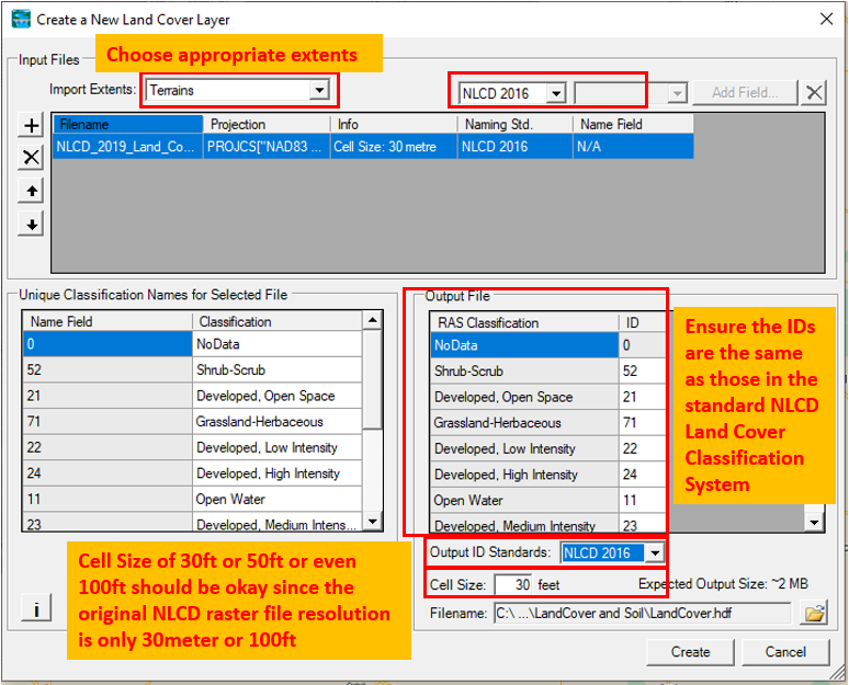
To start the process, download a NLCD raster file covering your project area from mrlc.gov/viewer and your state’s gSSURGO (geodatabase) in here. These two files do not need to be re-projected beforehand, and instead, RAS Mapper is able to recognize their projections (EPSG5070 Albers Equal Area) and re-project them automatically to the HEC-RAS project’s projection system when performing layer creations.

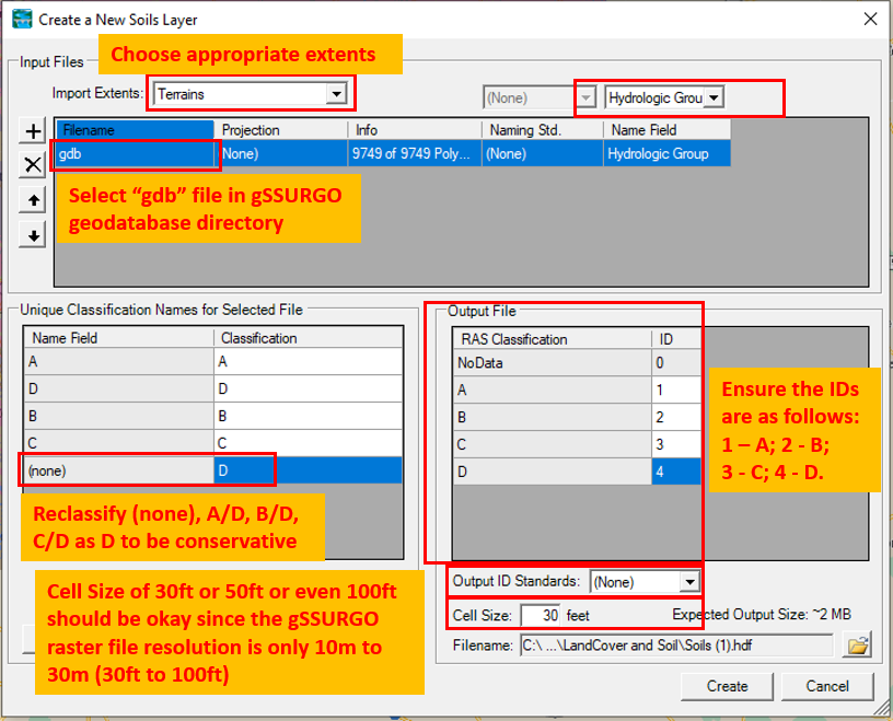
Import the NLCD raster file and the gSSURGO geodatabase file in RAS Mapper to create a Land Cover layer (Figure 3) and a soils layer (Figure 4).

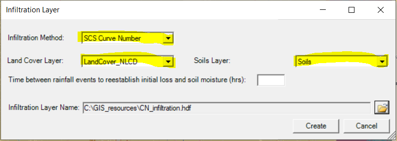
Now create an infiltration layer from Land Cover/Soils Layers (Figure 5) and assign Curve Number to different combinations of land covers and hydrologic soil groups (Figure 6 and Table 1).

Some of the curve numbers in Table 1 are meant to be composite values which have already included impervious area’s contribution. The Impervious area percentage should be set as 0.0 when applying these composite curve numbers; otherwise, the impervious area effect will be double-dipped. HEC-RAS 2D User’s Manual states “In practice, it is much more accurate to develop runoff Curve Numbers for the pervious area only and define the impervious area separately. In HEC-RAS, impervious area will be treated as 100% runoff with no infiltration. For example, this definition is especially important for urban areas, where runoff will occur at the very beginning of storms due to impervious areas that are directly connected to the storm runoff system“.

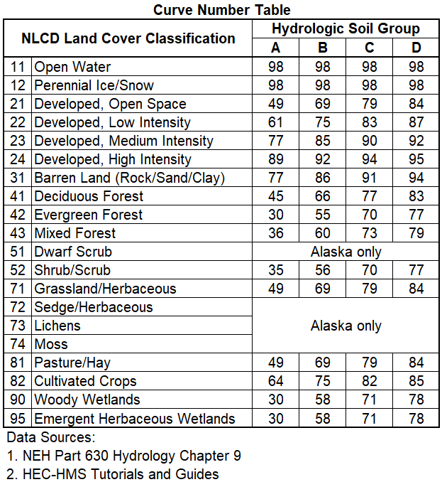
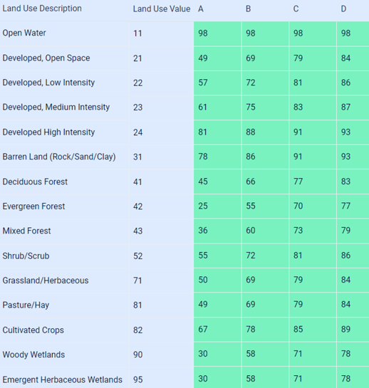
HEC-HMS Tutorials and Guides lists the curve numbers of various NLCD land uses (Table 2) which match the values in Table 1 closely.

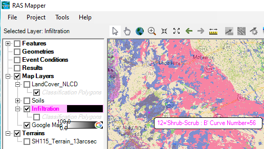
After entering curve numbers for the infiltration layer, their values can be viewed on RAS Mapper window by hovering the mouse cursor over any location on the map (Figure 7).

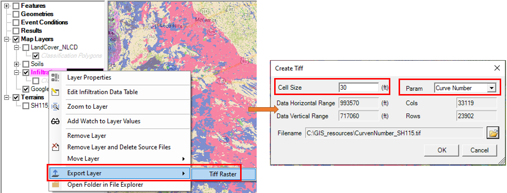
The infiltration layer created above can be exported as a raster file in RAS Mapper (Figure 8). Use HEC-RAS V6.1 to complete the exporting because it appears the HEC-RAS V6.4 or V6.5 does not support this function.

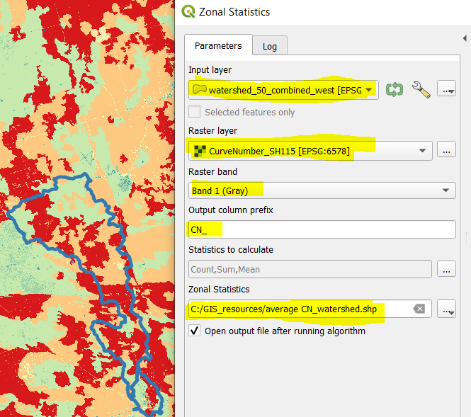
Utilizing QGIS (or ArcGIS) zonal statistics function, the average curve number for each watershed covered by the curve number raster file can be easily calculated (Figure 9) and the results are shown in Figure 10.

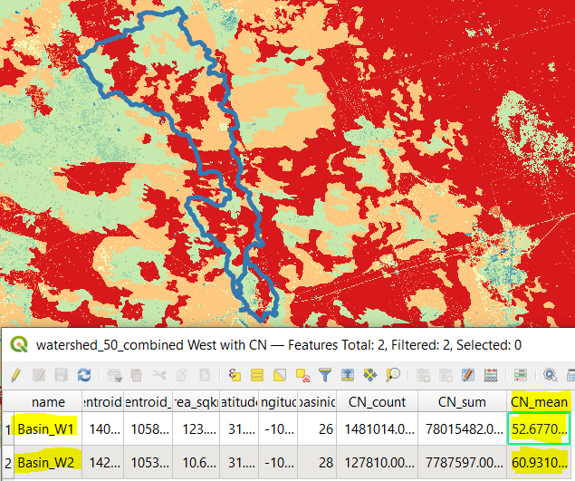
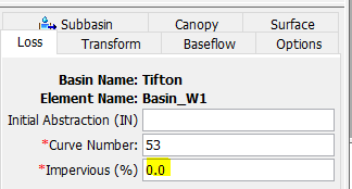
For Basin_W1 in Figure 10, its average Curve Number is about 53. Since the value of 53 is a composite curve number after taking into account impervious area effect, when modeling it in HEC-HMS, the Impervious (%) should be entered as zero (Figure 11).

The curve number raster file can also be imported to a HEC-DSS file via HEC-HMS Vortex Importer tool as a gridded curve number dataset (refer to the step by step instruction here).