Calculate Area-Weighted Average Curve Number Using Land Cover Raster File and HSG Raster File in QGIS (3 of 3)

This post (3 of 3) is an instruction of combining Land Cover Raster file and HSG Raster file to create a CN raster file for calculating an area-weighted average CN using QGIS spatial analysis function. For the previous instruction on how to generate a Land Cover Raster file, refer to the first post (1 of 3); for steps on creating soil HSG Raster file, see the 2nd post (2 of 3). Some example files used in the demonstration are listed at the end of this post for downloading if you are interested in them.

1. You should have a land cover raster file and a soil HSG raster file ready before combining them using GDAL Raster calculator of QGIS to create a CN raster file. It is important that the HSG raster file is generated by rasterizing the HSG shapefile using the same extent and resolution of Land Cover raster file as explained in the 2nd Post (2 of 3). Both files should be in the same projected coordinate system (EPSG 26917, UTM Zone 17N in the example).
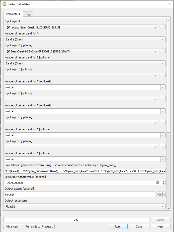
2. To create a CN raster file, search “raster calculator” in Processing Toolbox and select GDAL Raster calculator (Figure 1, Note: this is NOT the Raster Calculator… under top menu of Raster) and select Land Cover Raster file as Input layer A and HSG raster file as Input layer B. Copy the logic equation expression (the entire expression txt file can be downloaded here) into the field of Calculation in gdalnumeric syntax. The Output raster type is set to Float32 since the output raster is for CN. The output nodata value can be set to -9999 (or zero if you prefer). It should be emphasized that the logic equation expression is based on the Table 1 of the first Post (1 of 3). If you have different land cover reclassification and CN assignments, you should create your own logic equation expression for CN calculation. Actually you are encouraged to do so to fit your project requirements and needs.

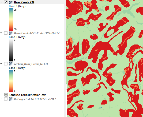
3. The calculated CN raster file is shown on Figure 2. The cell value of this raster file is CN.

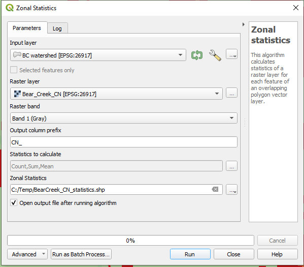
4. Load a watershed boundary shapefile to QGIS and open Zonal statistics tool (Figure 3). Pick Count, Sum, and Mean for Statistics to calculate and use “CN_” for Output column prefix.

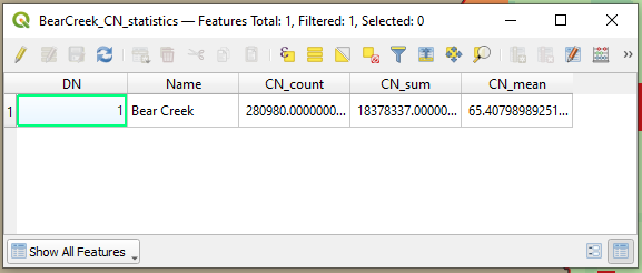
5. Three new fields are added to the watershed boundary shapefile as shown in Figure 4, where the value under the column of Mean is the area-weighted average CN (Mean is equal to Sum divided by Count). In this example, the area-weighted average CN (Mean) is 65.4.

Some example files used in the demonstration for downloading:

• Watershed boundary shapefile (zip file, EPSG 26917, UTM Zone 17N)
• Reclassified land cover raster file (EPSG 26917, UTM Zone 17N)
• Soil HSG code shapefile (zip file, EPSG 26917, UTM Zone 17N)
• Soil HSG code raster file (EPSG 26917, UTM Zone 17N)
• Logic Equation Expression for Calculating CN
• CN raster file (EPSG 26917, UTM Zone 17N)

Note: As of 2022, there is an easier way to create a curve number raster file in RAS Mapper – refer to this post.