Canopy Interception, Surface Storage, and Evapotranspiration (ET)
In addition to loss through infiltration, during a precipitation-runoff process other losses may need to be accounted for as well, which include canopy interception, surface depression storage, and evapotranspiration (ET). These losses are relatively small and thus often ignored in a single storm event modeling, however, for a continuous long-term simulation they can account for more than 50% of the total precipitations and usually should not be omitted.
Before becoming runoff or infiltrating into the soil, precipitation will first be intercepted by plant canopies and then be temporarily stored in surface depressions such as a puddle (Figure 1A). The intercepted or stored water can get lost to atmosphere through evaporation. The water stored in surface depressions can continue to infiltrate into the soil. The water in the soil will be absorbed by plant roots and released to air by plant transpiration (Figure 1B).
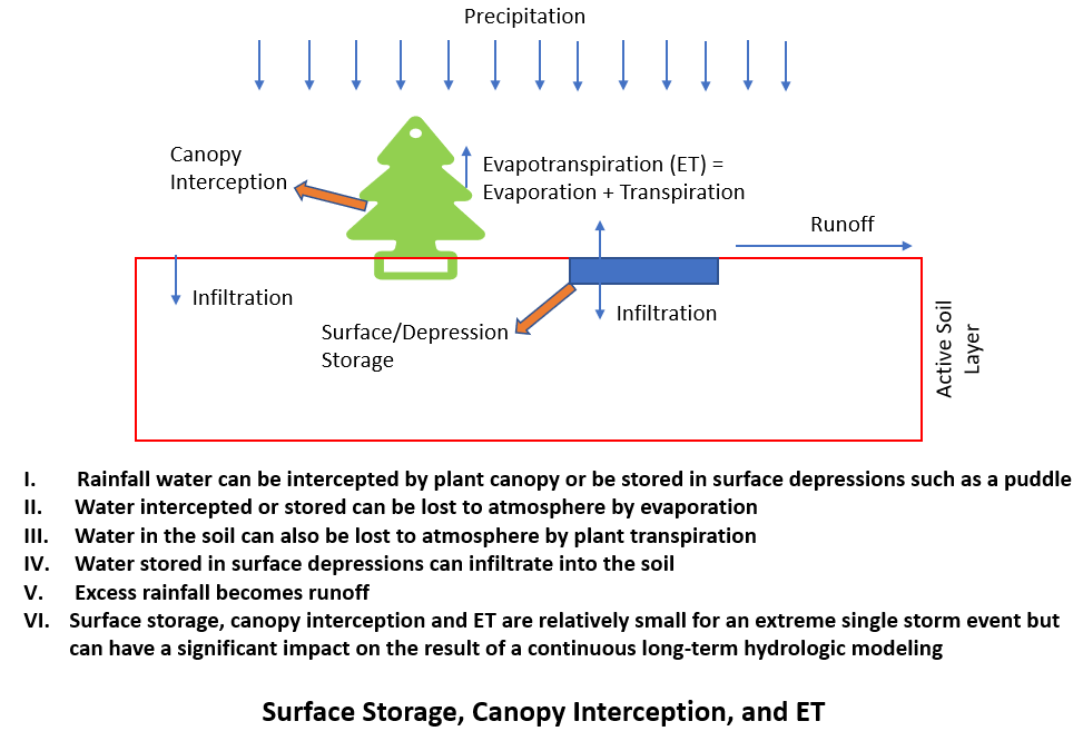
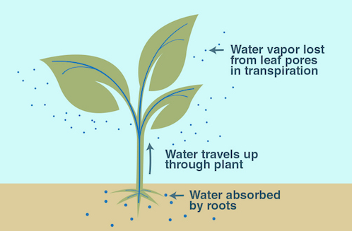
Table 1 summarizes some typical canopy interception and surface storage values for various plants and surface types. These values should be calibrated.

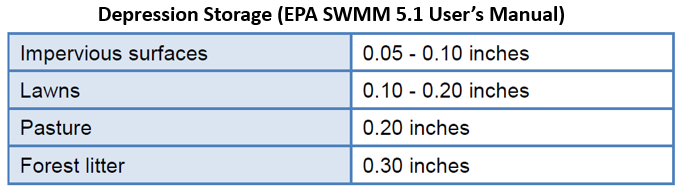
EPA SWMM 5.1 User’s Manual Appendix A.5 lists another set of depression storage values (Table 2), which are basically consistent with those in Table 1.
Attention should be paid to initial loss or depression storage when applying SCS Curve Number (CN) method to model infiltration loss: set initial loss as zero for SCS Curve Number method and use initial abstraction (Ia=0.2S by default) instead. Refer to this post for more discussions on SCS Curve Number (CN) infiltration method.
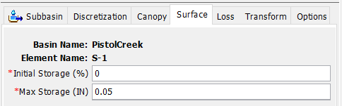
In HEC-HMS, two methods are available to account for surface storage: simple surface and gridded simple surface. The two methods are essentially the same except that the gridded simple surface method is to apply simple surface method on each grid cell. In Figure 2, Initial Storage (%) is the percentage of the maximum storage which is filled with water at the beginning of the simulation. Max Storage (IN) is the maximum amount of water that can be held on the soil surface before surface runoff begins (refer to Table 1 and Table 2 to estimate Max Storage).
Evapotranspiration is a term coined to represent evaporation from the ground surface/canopy and transpiration by plants since it is very difficult to measure and quantify these two processes separately. Through evaporation and transpiration water is returned from the surface and soil to the atmosphere. The evapotranspiration method is only necessary in a continuous long-term simulation in which the evapotranspiration will be used to calculate losses and reset soil water deficit.
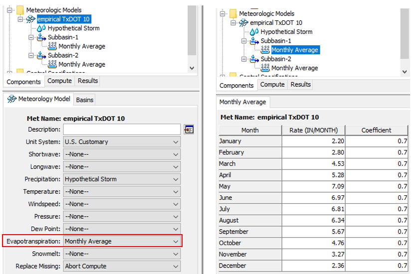
The potential evapotranspiration (ET), aka the theoretical evapotranspiration, serves as the upper limit for evapotranspiration rates based on atmospheric conditions. In HEC-HMS, the potential evapotranspiration is specified in Meteorologic Models. Monthly Average is one of the simplest ET methods in HEC-HMS (Figure 3). The total amount of evapotranspiration for each month is entered as inch/month (refer to the example values in Table 4). The pan coefficient of each month is to be provided as Coefficient in Figure 3. The final potential ET rate for each month is adjusted by the Coefficient. The potential ET volume is satisfied first from the canopy interception, then from the surface depression storage, and finally from the soil water content.
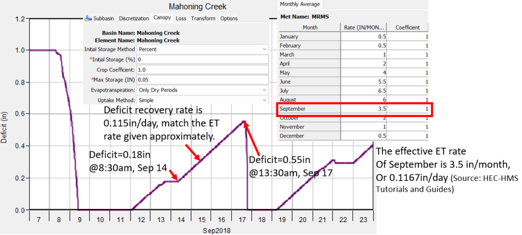
The canopy method is defined in subbasin elements in HEC-HMS. The most commonly used method, Simple Canopy is shown in Figure 4. The first two parameters (Initial Storage, and Max Storage – see Table 1) are to model canopy interception. The Crop Coefficient is a ratio applied to the potential ET rate when calculating the amount of water to be actually extracted from the soil. Apparently, a crop coefficient of 1.0 means the potential ET rate is applied directly without modification. The initial crop coefficient values can be set as 1.0 or estimated from Table 3 and then be adjusted during model calibration. The Uptake Method can be set as “Simple”, which depletes soil water content at “potential ET rate x Crop Coefficient” and usually is used together with the Deficit and Constant or Soil Moisture Accounting (SMA) loss methods to recover the soil water deficit during “dry” periods, as shown in Figure 5.

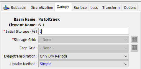
The Gridded Simple Canopy method implements the simple canopy method on a grid cell basis and each grid cell can have different Max Storage (Storage Grid) and Crop Coefficient (Crop Grid) (Figure 6).
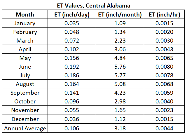
Robert Pitt summarized crop coefficients in Table 3 and ET values in Table 4 for the Cahaba River Experimental Watershed in central Alabama in the paper titled of “Evapotranspiration and Related Calculations for Bioretention Devices“. The paper includes another table for ET values of 18 subareas in California.

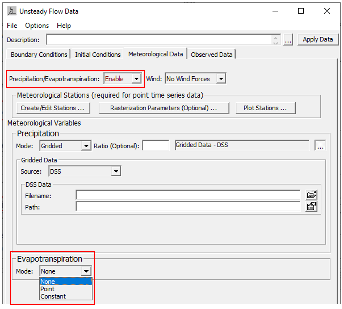
In HEC-RAS 6.1 the evapotranspiration data is required if a HEC-RAS 2D rain-on-grid (RoG) model needs to account for evapotranspiration loss to reset soil moisture deficit during “dry” periods. The evapotranspiration data is entered in Unsteady Flow Data Editor – Meteorological Data Tab (Figure 7) as point data, or a constant rate. It appears that the gridded data option for ET is not available in HEC-RAS 6.1 even though the 2D Users Manual claims so. Currently the evapotranspiration method can work with the Deficit and Constant or Green-Ampt infiltration method in a HEC-RAS 2D rain-on-grid model and they are optional.
USACE HEC has two presentations about the surface loss and evapotranspiration methods in HEC-HMS and they can be viewed here and here.
Leave a Reply