Initial and Constant & Deficit and Constant Loss Methods and Parameter Estimation

Initial and Constant Loss Method and Deficit and Constant Loss Method are two common infiltration methods in HEC-HMS and they share the same underlying concept, simply put, after the “initial loss” is met to saturate the soil layer, the following infiltration rate is constant which can be approximated as the soil saturated hydraulic conductivity. Unlike Green-Ampt method, their parameters are not easy to estimate, and therefore it is strongly recommended that any models utilizing these two loss methods shall be calibrated with monitored data.

Both methods are suitable in a single event HEC-HMS model, while Deficit and Constant Loss Method can also be used for a continuous simulation in which the soil water deficit can be recovered (or regenerated) during “dry” periods by Canopy Uptake and Evapotranspiration (ET).

To facilitate the discussion, some key terms are explained below.

• Porosity or Total Porosity: the fraction of the total soil volume that is taken up by the void space (Unit: dimensionless, V-void/V-bulk soil).
• Soil Water Content or Moisture Content: the fraction of the total soil volume is taken up by water. The corresponding value at the commencement of a simulation is called initial water content (Unit: dimensionless, V-water/V-bulk soil). The saturated water content can be estimated as total porosity.
• Field Capacity or Water Holding Capacity: the water remaining in a soil after it has been thoroughly saturated and then allowed to drain freely by gravity (taking one to several days). Usually it is measured as water content retained in soil at −0.33 bar of hydraulic head or suction pressure (Unit: dimensionless, V-water/V-bulk soil).
• Wilting Point:  the soil water content at which a plant can not absorb any more water and it starts to wilt since the water is held so tightly by the soil particles. Usually it is measured as water content at a soil matric potential of −15 bar (Unit: dimensionless, V-water/V-bulk soil).
• Available Water Content: water held in soil between its field capacity and wilting point (Unit: dimensionless, V-water/V-bulk soil) – available water content is usually used for irrigation and agriculture and it is not a common term in H&H modeling and engineering.
• Residual Water Content or Residual Moisture Content: the volumetric water content of a soil where a further increase in negative pore-water pressure does not produce significant changes in water content. It represents the remaining water content after a saturated soil is allowed to drain thoroughly for an extended period of time (Unit: dimensionless, V-water/V-bulk soil).
• Effective Porosity: usually the soil water content can not be zero: a realistic minimum soil water content can be defined as residual moisture content and thus, effective porosity = porosity – residual water content (Unit: dimensionless, V-void/V-bulk soil).
• Soil Water Deficit or Soil Moisture Deficit: the amount of water that is required to saturate the soil. The corresponding value at the commencement of a simulation is called initial deficit (Unit: inch).
• Maximum Deficit: the total or maximum amount of water that is required to saturated the soil when the soil is totally “dry” or at its minimum moisture content. The maximum deficit can be estimated as the product of active soil layer depth and effective porosity (Unit: inch).

The concept of the Initial/Deficit and Constant Loss Method is explained in Figure 1A. At the beginning of a rainfall event, the soil usually is not saturated and the precipitation (after surface/depression storage and canopy/evapotranspiration ) will penetrate the soil to fill the voids (Phase 1 and 2 in Figure 1A). When the soil becomes saturated (soil water deficit =0), the infiltrated water will percolate through the bottom of the active soil layer and get lost.

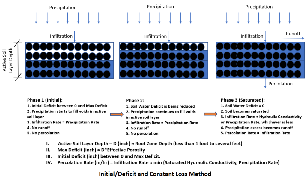
The required parameters of the Initial and Constant Loss Method are initial deficit (or initial loss, in inch) and constant rate (in/hr), while the Deficit and Constant Loss Methods also requires the maximum deficit (inch) in addition to the other two. The Initial and Constant Loss Method does not require the maximum deficit value since it is a single event method and the soil water content can not be depleted during the simulation.

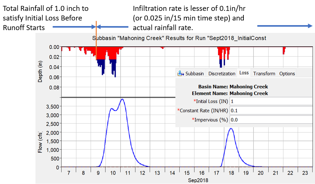
The rainfall and runoff graph from a HEC-HMS model using Initial and Constant Loss Method is shown in Figure 1B. The total accumulative rainfall depth is about 1.0 inch from the model beginning to 8:00am of September 9, 2018 to satisfy the initial loss; only after this time, the runoff starts and the infiltration rate is either 0.1 inch/hr or the actual rainfall rate, whichever is less.

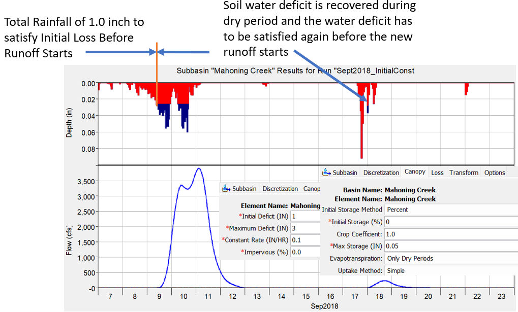
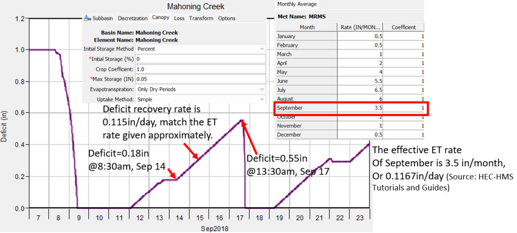
The same HEC-HMS model was revised by using Deficit and Constant Loss Method and defining a canopy and ET method. During the dry period between the two rainfall events, the soil water deficit is recovered so the soil becomes unsaturated. The resulted water deficit will have to be satisfied again before the second (new) runoff starts as illustrated in Figure 1C and Figure 1D.

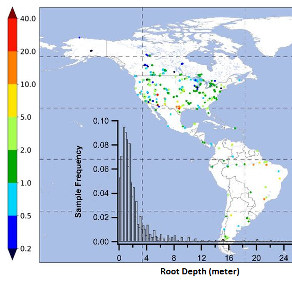
The active soil layer depth (D) is required to calculate initial deficit and maximum deficit as explained in Figure 1A. Usually the root zone depth can be used to approximate the active soil layer depth. Robert Pitt in the paper titled of “Evapotranspiration and Related Calculations for Bioretention Devices” shows root depth varies from 1.0 ft to 6.0 ft (Table 1). Ying Fan summarized 2200 observations of root depths and concluded that root depth varies from 0.01 meter to 70 meter with a distribution peak at 1.0 meter (Figure 2). Mean root depths of different soil textures and vegetations are also provided by Ying Fan in the same study (Figure 3 and Figure 4).

Under the field condition, it is common that the lower portions of the root zone are not active during the hydrology process and therefore the active soil layer depth can range from half of the root zone depth to the full root zone depth (less than 1 foot to several feet). For lack of a better estimation or guidance, the active soil layer depth may be initially estimated as a value between 1.0 and 2.0 ft after considering the fact that lower portion of root zone is often not active.

The initial deficit is the amount of water that is required to fill the voids in the soil at the commencement of a simulation and it is usually a value between zero (saturated) and maximum deficit (with residual water content). For a model to simulate a historical storm event, a practical way to estimate the initial deficit is to begin the simulation three days after the end of a previous precipitation event which has saturated the soil layer. Three days is the approximate time required for saturated soil to drain freely by gravity to a water content known as field capacity – in this case, the initial deficit can be estimated as the product of active soil layer depth and the difference between porosity (not effective porosity!!! – see Figure 5 for illustration) and field capacity, D * (porosity – field capacity). When simulating a historical storm event it is always a good practice to star the model run in advance enough from the time period of interest so that the modeling results are insensitive to the initial condition values.

Under the average antecedent moisture condition (average AMC), Dr. David Maidment in his book of Handbook of Hydrology suggested using wilting point (-1500 kPa water content) as initial water content in the western USA and using field capacity (-33kPa water content) as initial water content in the eastern USA. Correspondingly, the initial deficit will be calculated as D * (porosity – wilting point) for Western USA or D * (porosity – field capacity) for Eastern USA for average AMC. The typical values of (porosity – wilting point) or (porosity – field capacity) can be found in Table 2 of this post or Table 3 below.

The maximum deficit can be estimated as the product of active soil layer depth and effective porosity, or D * effective porosity. Some literatures suggest using D * (porosity – wilting point), however, since the realistic minimum soil moisture content is the residual moisture content, not wilting point which is defined as a water content limit meant for plants to absorb water, it is determined that “D * effective porosity” or “D * (porosity – residue moisture content)” is more reasonable to calculate the maximum deficit.

The constant infiltration rate in the Initial/Deficit and Constant Loss method can be initially estimated as the soil saturated hydraulic conductivity. In field, the constant infiltration rate tends to be less than the saturated hydraulic conductivity due to incomplete saturation at the bottom of the soil layer or root zone. For this reason, the constant infiltration rate may be reduced from its initial estimation during calibration. At each time step during a model run, the entered constant infiltration rate in HEC-HMS or HEC-RAS will be compared with the instant precipitation rate and the lesser of the two will be used to calculate the loss.

Some useful soil properties discussed above are summarized in Table 2 for the typical soil textures. The values in the table are taken from USACE EM 1110-2-1417, 1982 paper authored by Rawls et al, and 1983 paper authored by Rawls et al after unit conversion. Rawls stated in his 1983 paper that the Green-Ampt hydraulic conductivity is one-half the saturated hydraulic conductivity presented in the 1982 paper. For Initial/Deficit and Constant Loss Method, the hydraulic conductivity values from the 1983 paper (B) are recommended as the initial estimation of the constant infiltration rate, which is also endorsed by HEC-HMS Tutorials and Guides and EPA SWMM User’s Manual.

InfoWorks ICM has two options for rainfall-runoff process – the traditional subcatchment hydrology method and the Rain-on-Grid method. Currently as of 2021, the deficit and constant infiltration method can only be applied to the traditional subcatchment hydrology method, and it is not available for Rain-on-Grid.

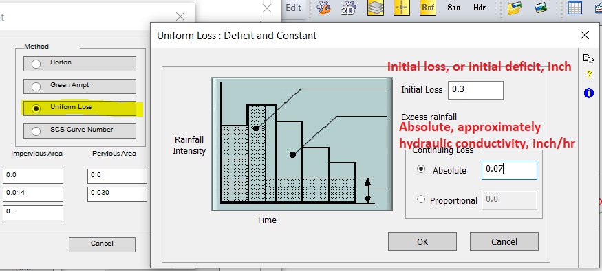
In XPSWMM, the initial and constant loss method is named as uniform loss (Figure 6).

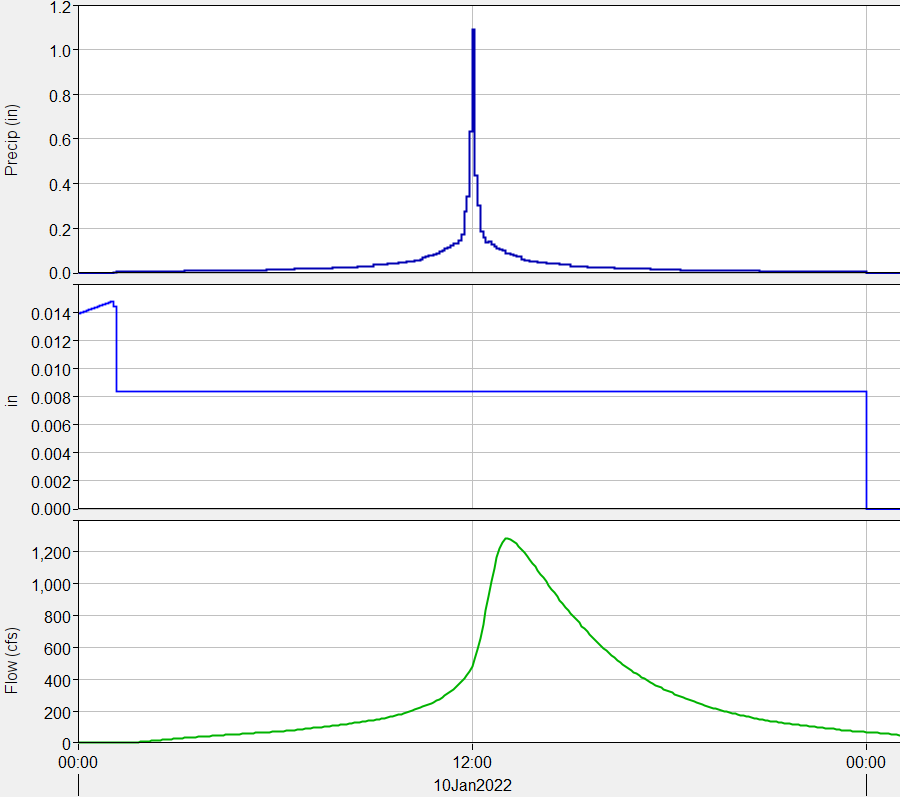
For illustration purpose, a HEC-HMS model result is shown in Figure 7 where the infiltration loss method is Initial and Constant.