HEC-HMS Hypothetical Storm Using NOAA Atlas 14 Precipitation-Frequency Grid and Point Depth
NOAA Atlas 14 provides the latest official U.S. precipitation frequency (PF) estimates for various durations and frequencies with lower and upper bounds of the 90% confidence interval. Refer to Post 1 and Post 2 for introductions on NOAA Atlas 14.
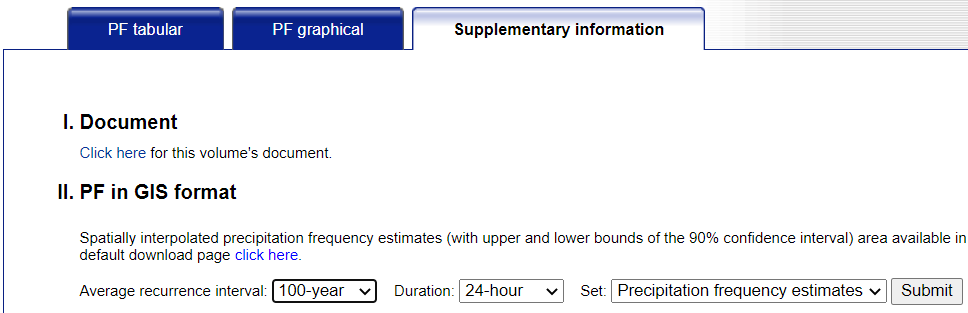
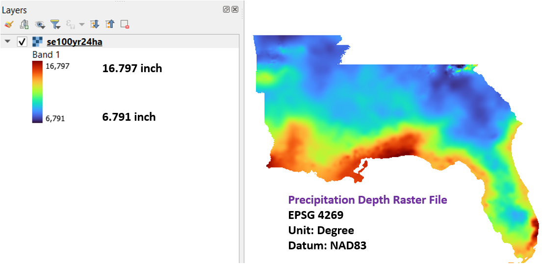
In addition to point precipitation depth and intensity data, a precipitation-frequency depth grid raster file can also be downloaded from NOAA PF Data Server (PFDS) for a selected frequency (AEP) and duration (Figure 1). The downloaded grid file (*.asc) is in EPSG 4269 with pixel values being scaled up by 1000. For this reason, in Figure 2 the precipitation depth ranges from 16.797 to 6.791 inch.
This post introduced a method to calculate area-weighted mean precipitation depths of different storm durations using the precipitation-frequency depth grid files and how to use these mean values to build a frequency storm in HEC-HMS. Alternatively, the precipitation-frequency depth raster file can be imported into HEC-HMS and be used as hypothetical storm when being supplemented with a cumulative precipitation depth distribution curve (percentage curve) and an area-reduction function/curve. The HEC-HMS subbasins need to be georeferenced in order to read the precipitation depths from the raster file.
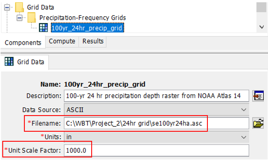
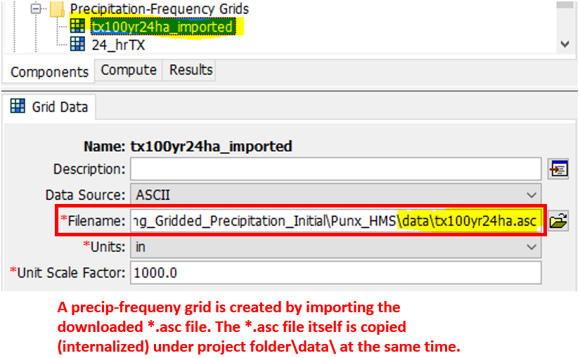
1. Create a precipitation-frequency grid using the downloaded precipitation-frequency depth raster file by clicking Components –> Grid Data Manager –> Precipitation-Frequency Grids (Figure 3A).
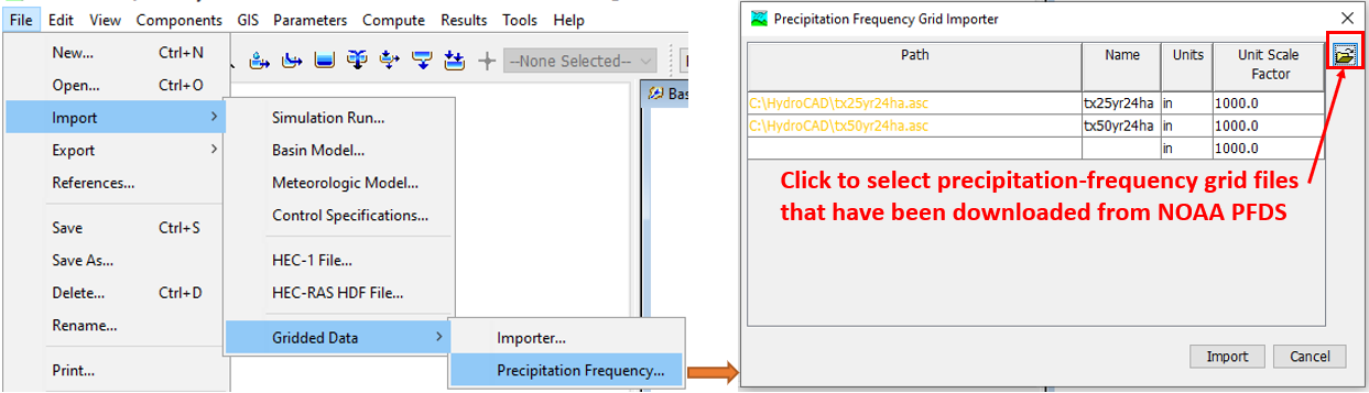
The latest version of HEC-HMS (V4.10 and later) supports importing the downloaded precipitation-frequency raster files to grid data directly by clicking File –> Import –> Gridded Data –> Precipitation Frequency… (Figure 3B and Figure 3C).
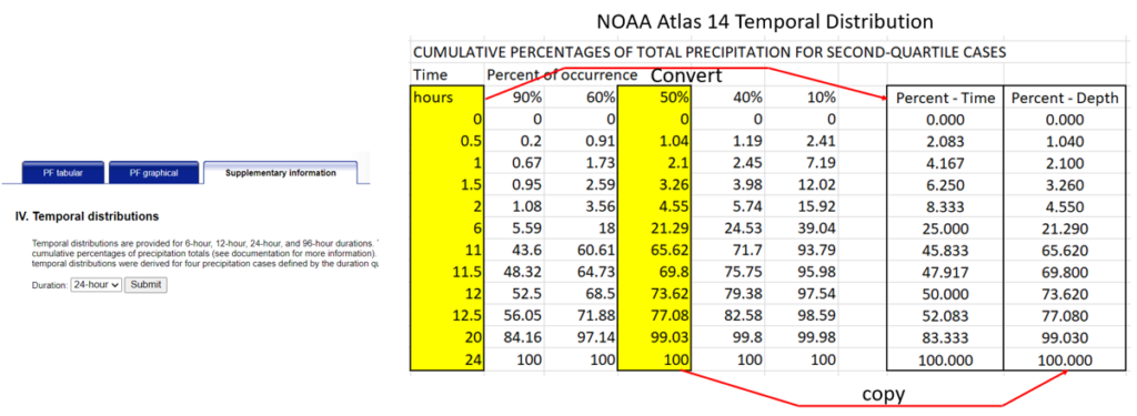
2. Create a percentage curve with dimensionless time Vs. dimensionless cumulative depth. The percentage curve is to define user-specified storm pattern, which can be a NOAA Atlas 14 temporal distribution, or any types of distributions.
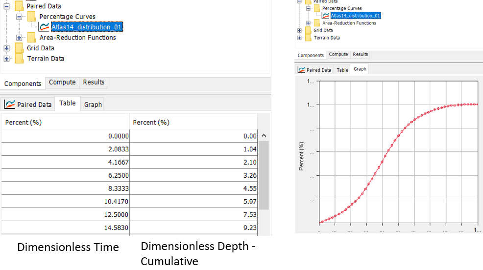
Figure 4 demonstrates how to download a 24-hr NOAA Atlas 14 temporal distribution and then convert it to a percentage curve in dimensionless time Vs. dimensionless cumulative depth format by using second-quartile 50% distribution curve data (refer to this post for details about NOAA Atlas 14 temporal distributions). The newly converted percentage curve can be imported into HEC-HMS as a set of paired data – percentage curves (Figure 5A).
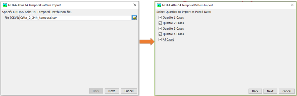
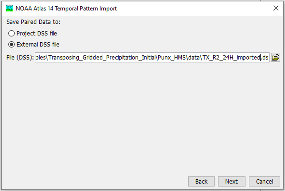
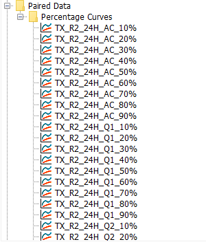
The new HEC-HMS also supports importing Atlas 14 Temporal Distribution *.csv files directly into HEC-HMS as paired data (percentage curves) by Tools–>Data–>Atlas 14–>Temporal Pattern Importer… (Figure 5B). The imported percentage curves are saved in a DSS file (Figure 5C) and viewable in HEC-HMS (Figure 5D).
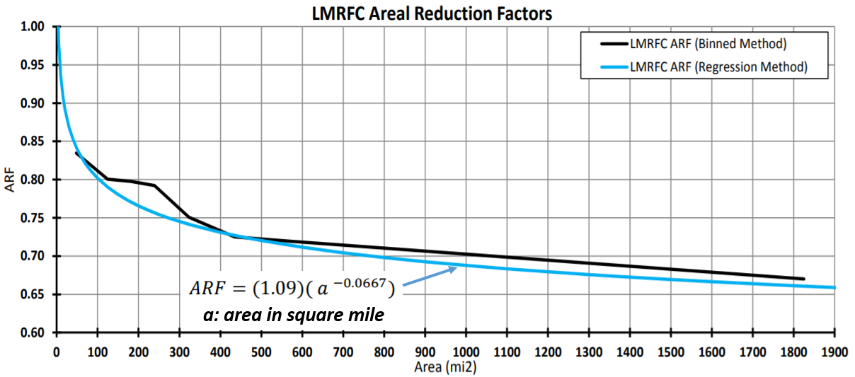
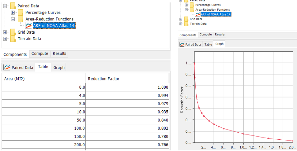
3. Optionally, create an area-reduction curve with the format of area (square mile) Vs. areal reduction factor. TP40 areal reduction factor is used commonly for storm durations up to 24 hours, which is explained here. Recently NOAA NWS completed a new study on areal reduction factors for Lower Mississippi in which a new areal reduction factor regression equation is presented (Figure 6). Apply the regression equation to create a set of the paired data – area reduction functions (Figure 7).
4. Create a hypothetical storm using data/curves from Step #1, #2, #3 above (Figure 8A). In Figure 8A, since the precipitation depth method is “Precipitation-Frequency Grid“, a modeler does not need to enter a point precipitation depth value, and instead, the program will automatically compute an average point depth value for the entire basin (Spatial Distribution is set as “Uniform For All Subbasins“) or each individual subbasin (Spatial Distribution is set as “Variable By Subbasin“). It should be noted that the Computation Point option is to be used when Spatial Distribution is set as “Uniform For All Subbasins“, in which the average point depth value for the entire basin is calculated based on the upstream watershed boundaries of the computation point; If Spatial Distribution is set as “Variable By Subbasin“, the average point depth value is calculated within each individual subbasin boundary and the Computation Point does not play a role at determining the subbasin average point depth.
Computation points can be managed through Parameters –>Computation Point Manager (or check out this post for more information about Computation Point). When a computation point is selected, you do not have to enter a storm area and the program will use the total upstream subbasin areas (determined by the areas covered by the subbasin georeferenced polygons, not the drainage area entered for subbasins) of the designated Computation Point to calculate the areal reduction factor. On the other hand, if a storm area is provided, the program will use the storm area for areal reduction factor computation.
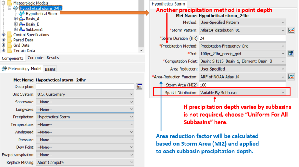
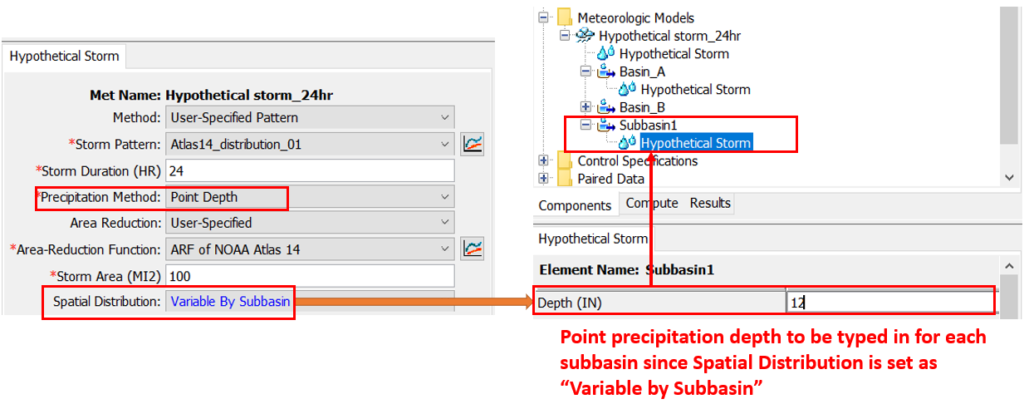
The hypothetical storm can also use point depth for precipitation method. The point depth method requires a modeler to manually type in a single point depth value for the entire basin or a unique point depth value for each individual subbasin if Spatial Distribution is set as “Variable By Subbasin” (Figure 8B).
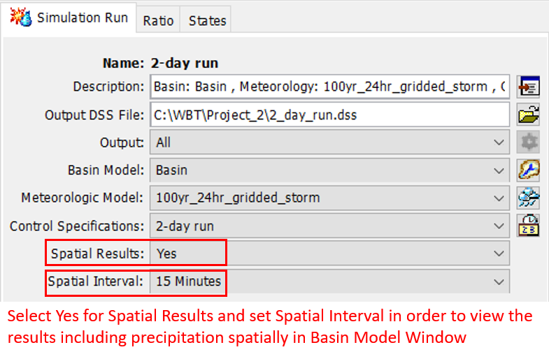
Run the HEC-HMS model using the hypothetical storm created above. In addition to the common result view options such as hydrographs and time series tables, the results can be viewed spatially if select “Yes” for Spatial Results in Simulation Run editor (Figure 9 and Figure 10).
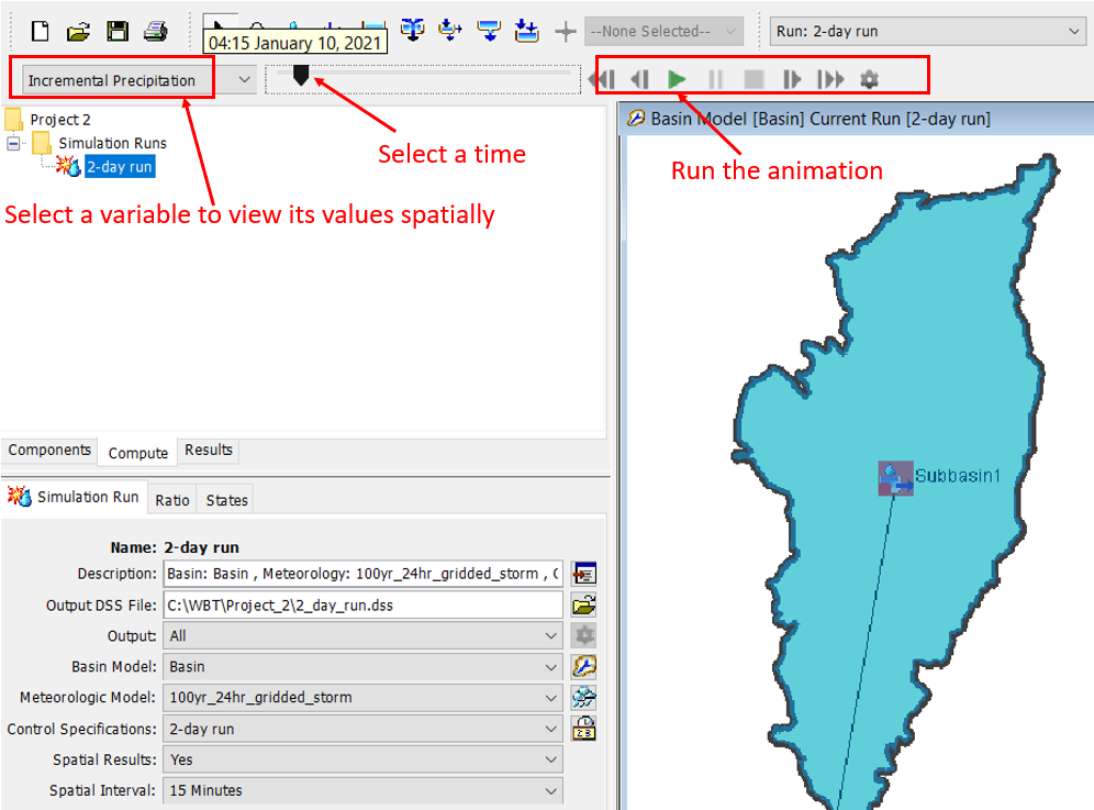
It is worth noting that the hypothetical storm created from gridded precipitation depth rater file is NOT a spatially varying storm; instead, HEC-HMS takes the mean value of depths over each subbasin and then applies a single storm distribution to the entire subbasin.
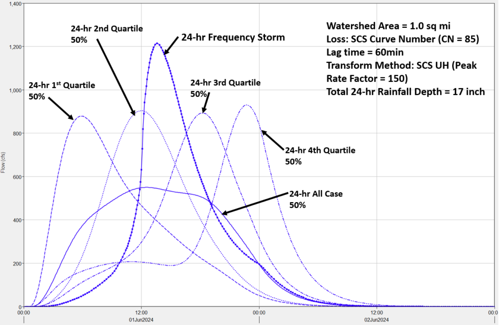
A HEC-HMS model was established to compare the runoffs between using frequency storms and the Atlas 14 temporal rainfall distribution. As shown in Figure 11, the frequency storm resulted in the greatest peak flows while the 24-hr all case 50% temporal distribution had the lowest peak flow. The other four Atlas 14 temporal distributions (1st quartile to 4th quartile 50%) ended up with peak flows that are very close.
Leave a Reply