XPSWMM Confusions and Clarifications (1 of 2)

XPSWMM is a popular 1D and 2D hydrologic and hydraulic modeling tool developed by Innovyze. Though originally XPSWMM was designed primarily to model storm sewer network system, it has gained the capability to model open channels, rivers, 2D overland flows and 1D-2D coupled systems in recent years. This post is 1 of 2 posts to clarify some topics that quite often confuse new XPSWMM users (for other topics covered by Post 2 of 2 click here). Note that sanitary sewer modeling is not covered by either post.

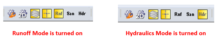
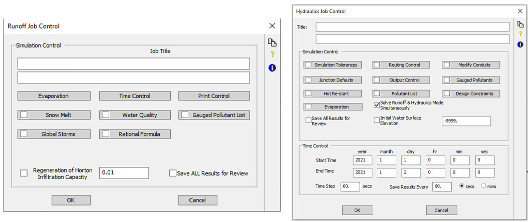
1. XPSWMM has two basic modes: runoff mode and hydraulics mode, which are inherited from the historical EPA SWMM RUNOFF and EXTRAN blocks. XPSWMM runoff mode and hydraulics mode can be turned on or off by clicking the tool bar icon Rnf and Hdr (Figure 1). Runoff mode and hydraulics mode have their respective Job Control setups (Figure 2).

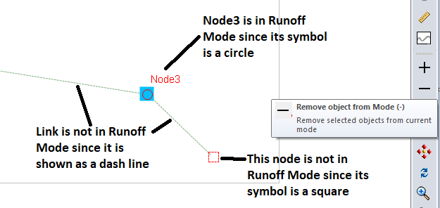
2. A node or a link can be added or removed from any mode by using the “+” and “–” tool on the right side of the main XPSWMM window (Figure 3). Usually a node should be added on to runoff mode if it receives runoff flows from a catchment in XPSWMM; otherwise, it should be removed from runoff mode; A link probably should only belong to hydraulics mode.

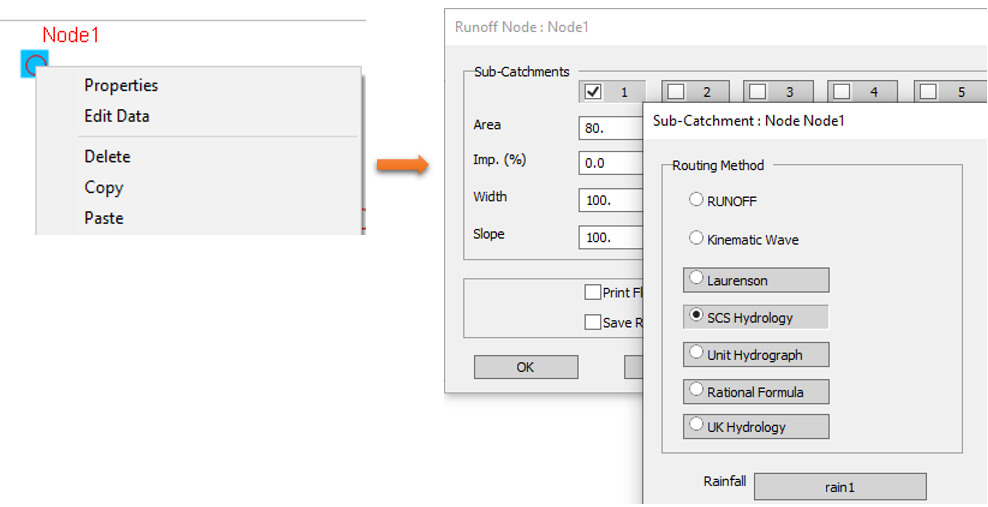
3. A catchment element is really not a must for a node to receive runoff flows in XPSWMM. If drainage areas have been delineated by GIS or other tools and the hydrology parameters are calculated outside XPSWMM, simply right click a node and then choose “Edit Data” to type in its hydrology/runoff calculation required parameters as shown in Figure 4. There is no catchment element involved in this process.

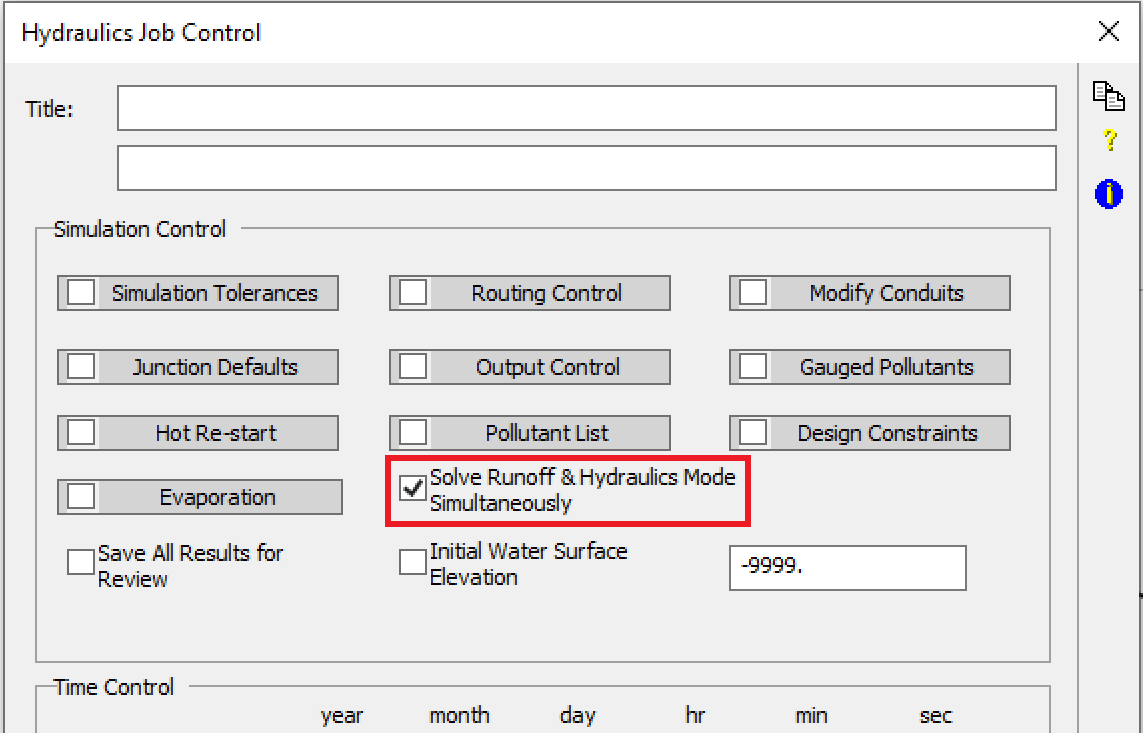
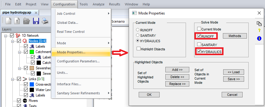
4. Historically EPA SWMM (up to SWMM4) conducted runoff and hydraulics calculations separately in RUNOFF, TRANSPORT, and EXTRAM blocks and the results of RUNOFF block is transferred to TRANSPOR/TEXTRAN blocks through interface files. Although XPSWMM inherits this feature, it is always recommended to calculate runoff and hydraulics simultaneously in current XPSWMM versions unless a modeler has a special need to use interface files to transfer results. To set up runoff and hydraulics calculation to run concurrently, first to check on the option of “Solve Runoff & Hydraulics Mode Simultaneously” in Hydraulics Job Control (Figure 5); and secondly, enable both RUNOFF and HYDRAULICS in Mode Properties setting (Figure 6).

5. Both runoff mode and hydraulics mode have their own time controls (start date and time, end date and time). When XPSWMM is set up to solve runoff mode and hydraulics mode simultaneously, it simply applies the instantaneous results of runoff mode to hydraulics mode without checking whether their respective year/month/day match or not (it appears XPSWMM does check runoff and hydraulics start time’s hour values), and for this reason, it is a good practice to keep them the same as shown in Figure 7 to avoid any confusions. It should be noted that the time steps of the two modes can be different and usually hydraulics mode requires a much smaller time step due to model stability requirement.

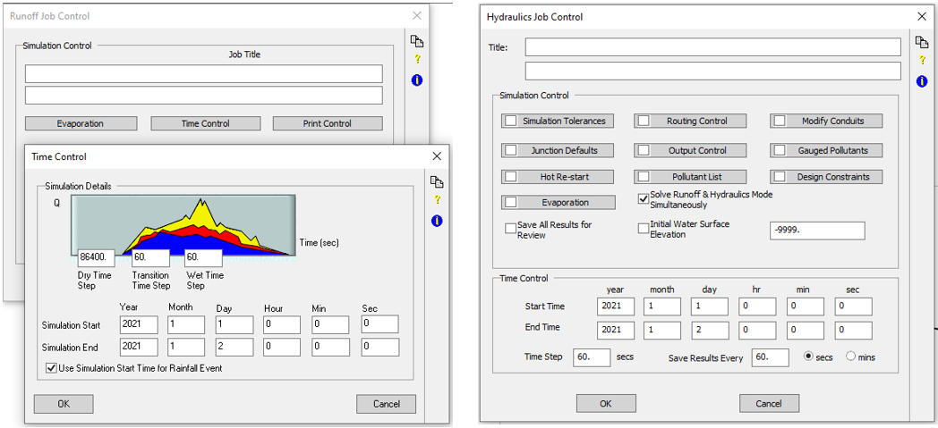
It is worth noting that the time step of Hydraulics Job Control is the maximum allowed time step; when XPSWMM solves a model, the actual time step will be based on courant number and no less than MIN_TS (by default MIN_TS=1.0 sec, but it can be overridden to a smaller number such as MIN_TS=0.2 in Configuration Parameters).

It is highly recommended that the start time is set to be zero (0.0) hour (midnight) of a day for both runoff and hydraulics time control, even though XPSWMM allows a non-zero hour start time. When a user supplied inflow or stage hydrograph (hours: flow in cfs or hours: stage in ft) is defined in XPSWMM, its zero (0.0) hour is meant to be at midnight on the starting day of the simulation. For this reason, if a hydraulics job control start time is non-zero, for example, set it at 5 (am), XPSWMM will only read the user defined inflow or stage hydrograph from 5.0 hours and ignore values from 0.0 hour to the time before 5am.

Using interface files to transfer data between runoff mode and hydraulics mode is a different story: XPSWMM will check data and time to make sure they match before applying runoff mode results to hydraulics mode.

6. Water can only be lost through nodes in XPSWMM due to flooding or surcharge (Figure 8) and water loss does not happen within a link.

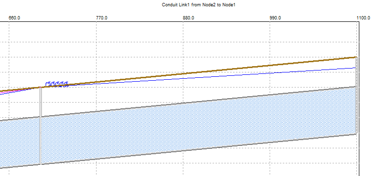
6. In XPSWMM, the HGL of a link is NOT calculated within the link, but assumed as a straight line connecting the water head of the upstream and downstream nodes. For this reason, if a link (pipe) is too long or the length is not that long but the slope is very steep, you may want to add additional “dummy” nodes to divide the link into multiple shorter ones to get better and more realistic HGL results. Adding additional “dummy” nodes may also help increase a model’s numerical stability.

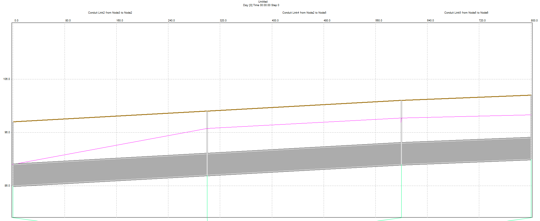
7. A detention pond can be modeled as a storage node in XPSWMM with the storage node depth being measured from “Node Invert” and the ponding option being “None” or “Allowed” (Figure 10).

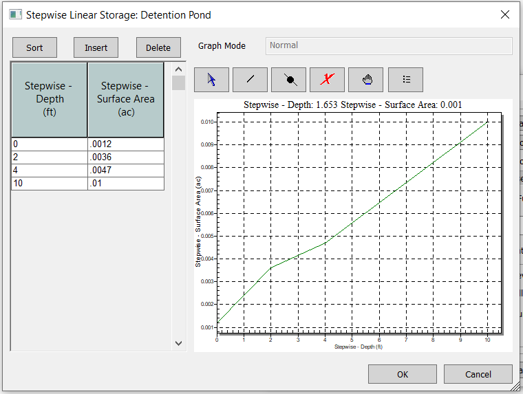
The spill crest can be set as the actual detention pond top of bank elevation, in this example of Figure 10, it is at Elev 100. Since the pond is 10ft deep (100-90=10.0ft), its stepwise linear storage paired data is entered from depth of 0.0 to depth of 10.0 as shown in Figure 11. If the modeled depth is greater than 10 ft in the pond (above Elev 100), XPSWMM will re-use the last surface area by assuming a vertical wall surrounding it to calculate its values. Of course, a modeler can always provide an artificial high value to ensure the entered maximum depth is always larger than the modeled depths. Usually the Surcharge Elevation option should be set as “Use Spill Crest Elevation“, and otherwise the storage method will only work when water level is below this surcharge elevation; above it, the surface area of the node is the default manhole surface area.

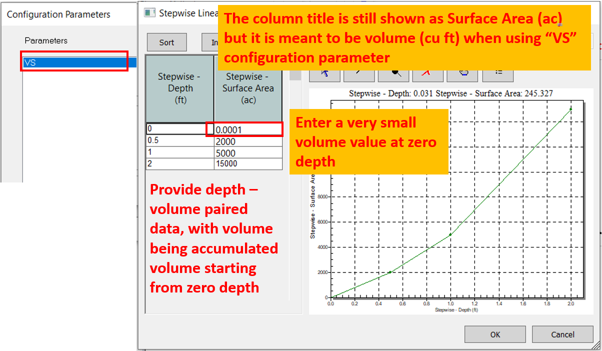
The default stepwise linear storage method requires a paired data set of depth and surface area, however, if desired, a modeler can override the program setting using “VS” configuration parameter to enter depth and volume values (Figure 12).

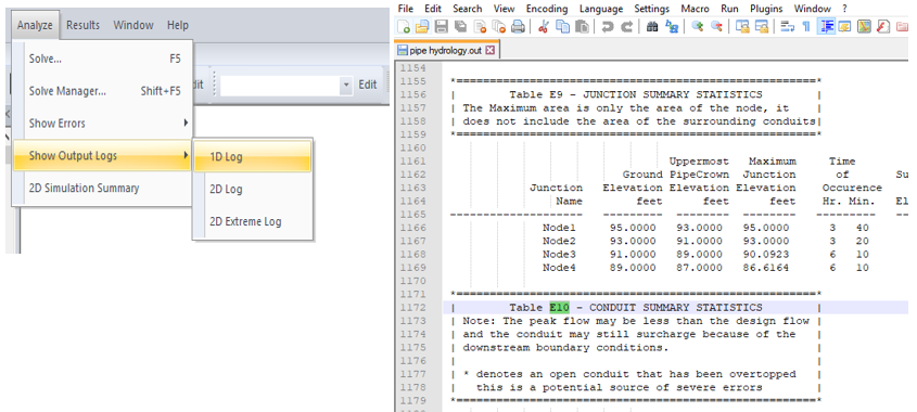
8. After each successful model run, a detailed output log can be reviewed by clicking Analyze—>Show Output Logs—>1D Log or 2D Log or 2D Extreme Log as shown in Figure 13.

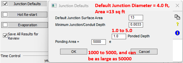
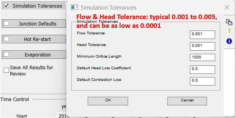
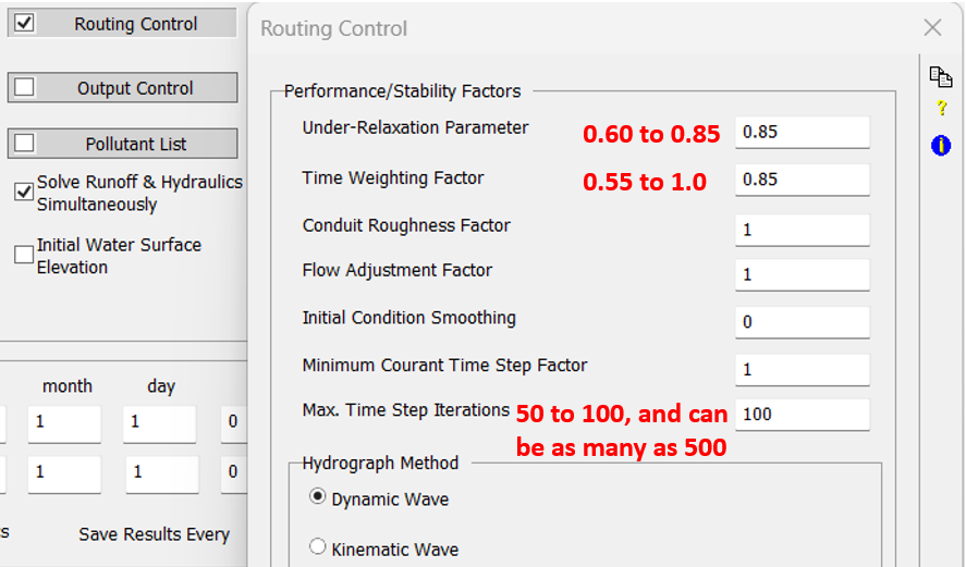
9. Pay attention to some job control settings in Hydraulics Mode. Some typical values are shown in Figure 14 , Figure 15, and Figure 16 for Junction Defaults, Simulation Tolerances and Routing Control.