XPSWMM Confusions and Clarifications (2 of 2)

XPSWMM is a popular 1D and 2D hydrologic and hydraulic modeling tool developed by Innovyze. Though originally XPSWMM was designed primarily to model storm sewer network system, it has gained the capability to model open channels, rivers, 2D overland flows and 1D-2D coupled systems in recent years. This post is 2 of 2 posts to clarify some topics that quite often confuse new XPSWMM users (for other topics covered by Post 1 of 2 click here). Note that sanitary sewer modeling is not covered by either post.

1. There are two ways to model dual-pipe, or multiple- pipe system between two nodes (such as double box culvert) in XPSWMM.

• Set the Number of Barrels to 2 or whatever the total number of parallel pipesbetween two nodes in Conduit Factors setting window (Figure 1A). To use this option, the multiple pipes must possess the same sizes, materials, and upstream/downstream flowlines.

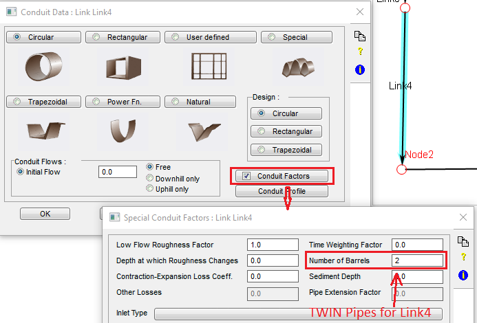
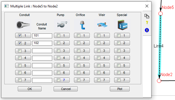
• Use the Multi-link option of XPSWMM to set up multiple parallel pipes between two nodes. (Figure 1B). The pipes do not have to be the same size and flowlines as required by the first option. This option has more flexibility for modeling and it is the recommended method for multiple-pipe modeling in XPSWMM.

2. Model culverts in XPSWMM: to turn on culvert calculation routine in XPSWMM, click and check on “Conduit Factors” option in Conduit Data Edit window, and select Inlet Type for inlet control calculation and provide Entrance Loss and Exit Loss Coefficients for outlet control calculation as shown in Figure 2. The Entrance Loss Coefficient can be found at Table C.2, Appendix C of HDS-5. The Exit Loss Coefficient usually is 1.0 and it can vary between 0.3 and 1.0 per HEC-RAS Hydraulic Reference Manual. Refer to this post for more information about culvert modeling by XPSWMM and other tools.

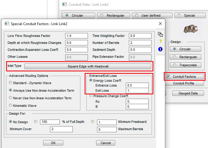
When modeling a storm sewer pipe, the entrance loss and exit loss into/out of a manhole are often ignored. Occasionally they may need to be modeled, but keep it in mind that the entrance loss and exit loss coefficients are not the same ones as those for culverts. Refer to this post for more information.

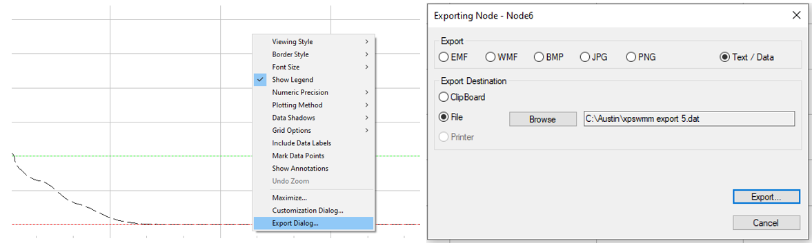
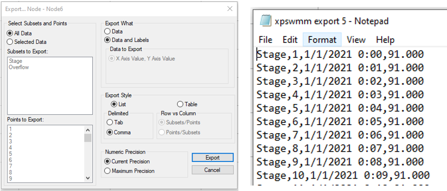
3. To export modeling results as time series data, right click a node or link’s graphic result view window and open “Export Dialog…” to choose Export File type as Text/Data and pick a file name and location (Figure 3A). In the next window, various export file options are available for selecting (Figure 3B). Usually it is just convenient to save the file as a CSV file (Delimited by Comma) which can be opened and edited by Notepad or Excel. In Figure 3A, if the Export Destination is “Clip Board“, the exported data can just be pasted to a blank excel file.

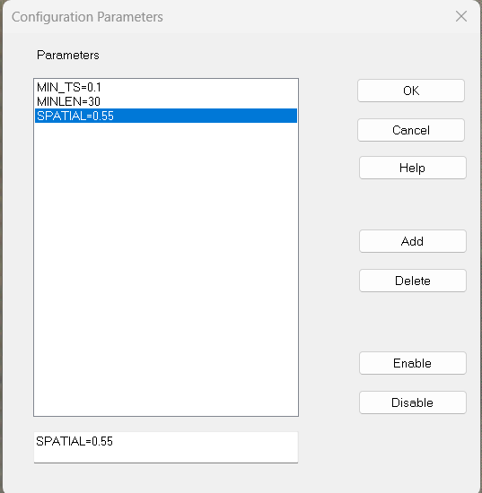
4. XPSWMM has various configuration parameters which control how a model is solved mathematically. The default values of a model’s configuration parameters can be viewed in its 1D log file after a successful model run (Figure 4A).

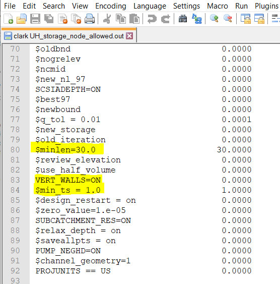
In Figure 4A, some parameter names start with “$” which means they are the XPSWMM default values. The default values can be overridden in Configuration Parameters window under “Configuration” menu (Figure 4B). MIN_TS and MINLEN are two common parameters that a modeler should pay attention to when dealing with model numerical stability issues. Another parameter, SPATIAL, probably should be overridden to 0.55 from its default value of 0.90 per XPSWMM manual.

5. Node Spill Crest Elevation for Open Channel: setting spill crest elevations for nodes connecting an open channel can become tricky. First of all, it should be noted that XPSWMM was originally developed to model a closed pipe network and therefore there are limitations on open channel modeling by XPSWMM, for example, there is no actual node for a river, but in XPSWMM river segments have to be connected by nodes just like a closed pipe system. Furthermore, when a river is overtopped, water will be lost from the lowest points of river banks in a real world, but in XPSWMM, water can only get lost through nodes. There are several scenarios for setting up node spill crest elevations of nodes connecting an open channel or a river:

• 5.1 – If we assume the water above the top of cross section will be lost from the system, set up the node spill crest at the same elevations as the top of channel cross section and the ponding option of the node will be “None“. Or, if you want to store the lost water in the system for it to return to nodes/river at a later time, enable the ponding option.

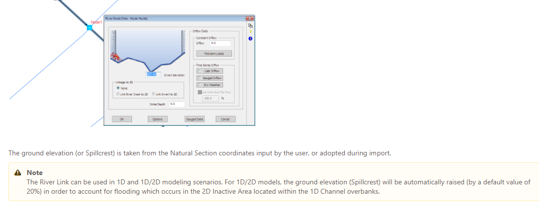
• 5.2 – If we want to keep the water above the top of cross section (top of bank) in the system, set up the node spill crest at a higher elevation than the top of channel cross sections. When overflow happens, XPSWMM by default will assume a vertical wall on both sides of the cross section and the water in the open channel can rise all the way up to the upstream/downstream node spill crest elevation but is contained by the vertical walls (Figure 5A). VERT_WALLS=ON does not need to typed in manually in Configuration Parameters since it is XPSWMM’s default setting. In an 1D-2D coupled system where an 1D open channel is connected hydraulically to 2D overland areas, the node spill crest is usually set to an elevation higher than top of cross section so that the 1D open channel water surface can rise above top of cross section (top of bank) to mimic flooding, which would also allow flood water exchange with 2D overbank areas. For a river link’s node when being modeled in an 1D-2D coupled system, the spill crest elevation will automatically be raised by 20% in order to account for flooding (Figure 5B).

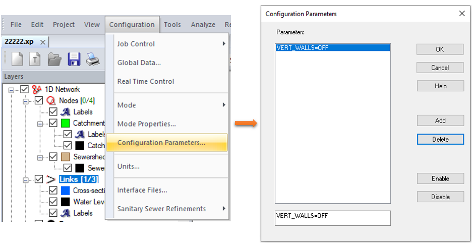
• 5.3 – If we don’t wish the water in Scenario 5.2 to raise above top of bank, the default vertical wall option can be turned off by typing in VERT_WALLS=OFF manually in Configuration Parameters (Figure 5C). This configuration is like to put a lid on top of the open channel and it can effectively set the open channel under pressurized flow (water will still rise in the nodes to push water through the lidded open channel, but the water in the channel will not rise above top of the bank due to the imaginary lid). Scenario 5.3 should be used rarely in XPSWMM modeling unless you need to model the open channel as a bridge.

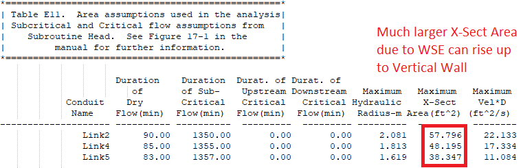
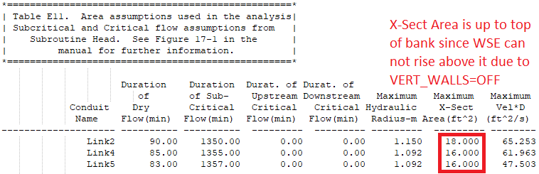
The difference between Scenario 5.2 and 5.3 can be confirmed by checking the E11 Tables of the output log files. In Scenario 5.2, water in the open channel can rise above top of the bank so the X-Sect Areas are pretty big (Figure 5D); while in Scenario 5.3, water in the open channel is confined by the imaginary lid and flow in the open channel is pressurized and therefore the X-Sect Areas are only up to the top of the bank (Figure 5E).