Calculate Area-Weighted Average Curve Number Using Land Cover Raster File and HSG Raster File in QGIS (2 of 3)
Hydrologic Soil Group Data (A, B, C, and D) is an important soil property which impacts the soil infiltration rates and runoff potential. Soils were originally assigned to hydrologic soil groups based on measured rainfall, runoff, and infiltrometer data. Hydrologic Soil Group Data (HSG) is included in SSURGO (Soil Survey Geographic database) which is distributed by the Natural Resources Conservation Service (NRCS) of USDA. NRCS provides two ways to download an area’s SSURGO: One is through Web Soil Survey to download SSURGO as shapefiles and tables and the other is through NRCS’s Data Gateway to download SSURGO as geodatabase.
This post (2 of 3) is on how to download SSURGO from Web Soil Survey (EPSG 4326) and how to process the raw data downloaded to generate a HSG Shapefile and Raster File. A HSG raster file can be used together with a land cover raster file (refer to Post 1 of 3 on how to create a land cover raster file) to create a CN raster file for calculating area-weighted average CN – this process is illustrated in this post (3 of 3). Some example files used in the demonstration are listed at the end of this post for downloading if you are interested in them.
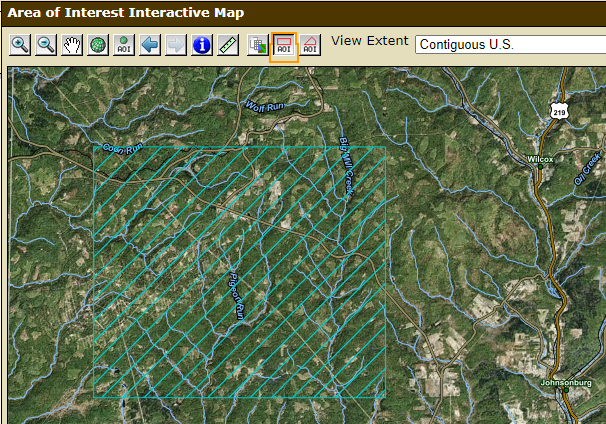
- Go to Web Soil Survey website to set area of interest (AOI) by drawing a box as boundary (Figure 1) or upload a boundary shapefile .
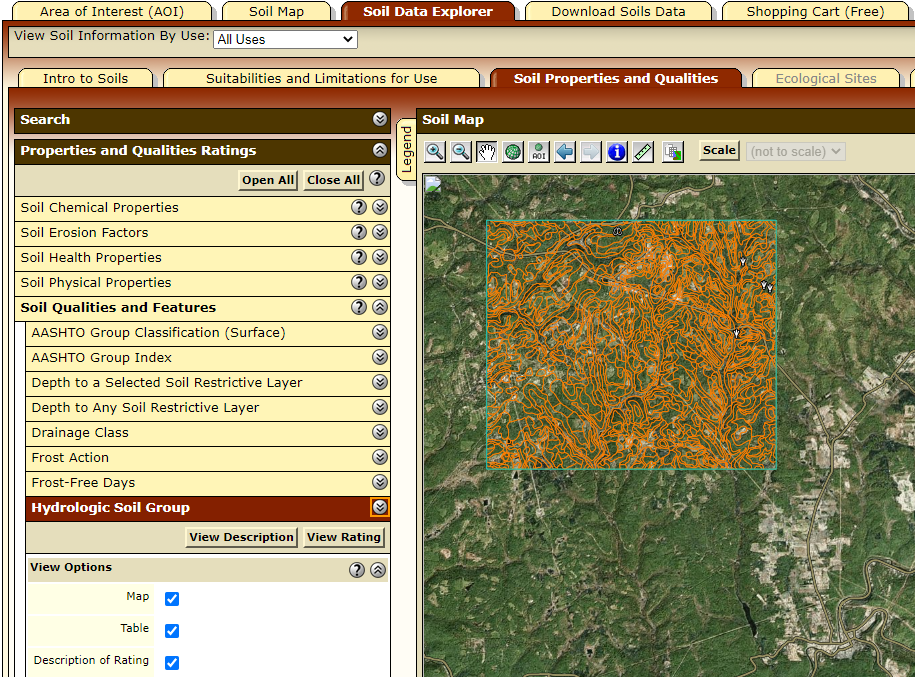
- On the top of the screen, click the tab of Soil Data Explorer and then its sub-tab of Soil Properties and Qualities. Expand the list of Soil Qualities and Features on the left and select Hydrologic Soil Group (Figure 2).
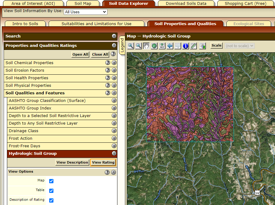
- Click “View Rating” button under Hydrologic Soil Group on Figure 2, the soil map view changes to show HSG map (Figure 3)
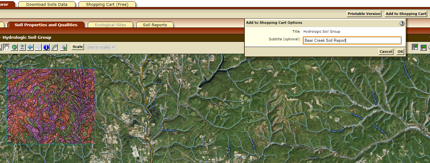
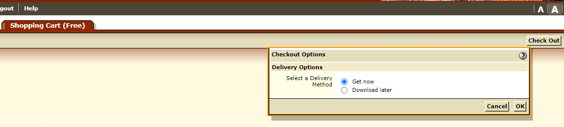
- Optional step: to create a soil report in PDF format for the AOI, click Add to Shopping Cart on the upper right of the screen (Figure 4) and type in the Subtitle as you like and click OK. Click the top tab of Shopping Cart (Free) to go to shopping cart page. On the shopping cart page (Figure 5), click Check out and select Get now to generate a soil report for download. You can download a sample soil report here.
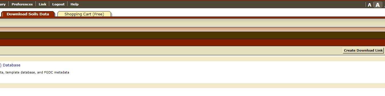
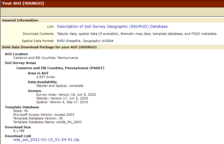
- Click the top tab of Download Soils Data to go to soil data download page. Click Create Download Link on the upper right of the screen (Figure 6) and the download link will appear at the bottom of the screen (Figure 7).
- Click the Download Link to download SSURGO data of your AOI which includes HSG data (Figure 7).
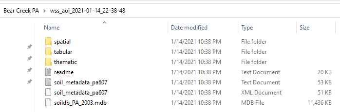
- Unzip the downloaded zip file and the folder structure is shown on Figure 8.
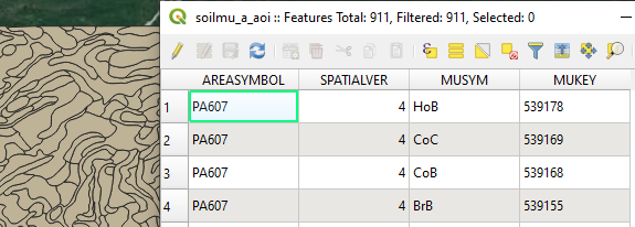
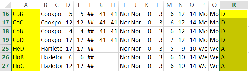
- Load the shapefile soilmu_a_aoi.shp under the folder of spatial into QGIS and open its attribute table (Figure 9). It can be seen that the shapefile does not have a field (column) of HSG (A, B, C, or D), and instead, it is using Map Unit Symbol MUSYM for different soils and each MUSYM code (example: HoB, CoC) can be linked to a certain HSG (A, B, C, and D) by using the table of muaggatt.txt under the folder of tabular (Figure 10). In Figure 10, muaggatt.txt is opened by Excel as a Delimited File using Vertical Bar “|” as delimiter, and the first column (A) is MUSYM code and the 18th column (R) is HSG (A, B, C, and D).
- To joint the table muaggatt.txt to soilmu_a_aoi.shp and impart its HSG field soilmu_a_aoi.shp:
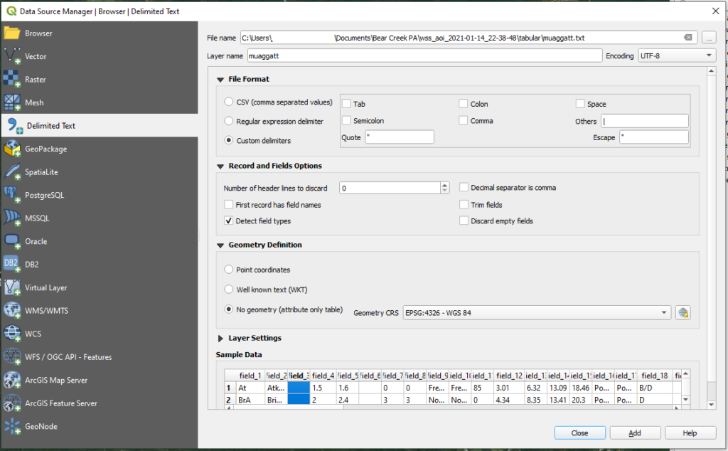
- Open Data Source Manager – Delimited Text (Figure 11) and select file of muaggatt.txt. Set File Format as Custom delimiters (Vertical Bar “|”) and No geometry. Click Add to load the table to QGIS.
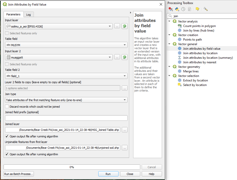
- Open Processing Toolbox, Search and open Join attributes by field value (Figure 12) to add the table muaggatt.txt‘s field_18 (HSG data) to a newly generated shapefile HSG_Joined Table.shp. Select MUSYM for Input Layer (soilmu_a_aoi.shp) Table field and field_1 for Input Layer 2 (muaggatt.txt) Table filed 2. Choose field_18 for Layer 2 fields to copy.
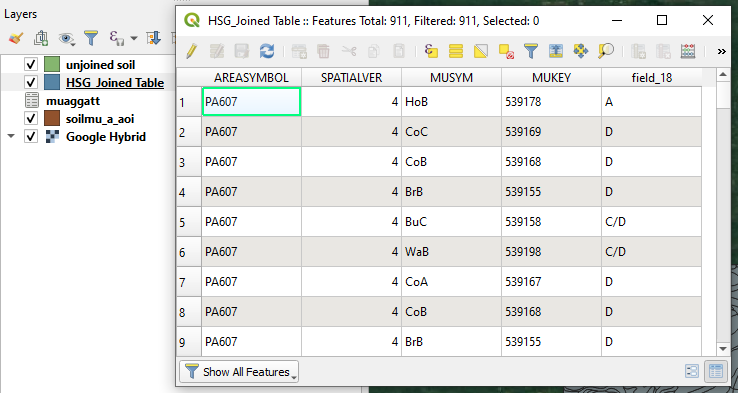
- Open HSG_Joined Table.shp attribute table to confirm field_18 is added (Figure 13).
Now let’s create another HSG shapefile with A, B, C, D being coded as 1, 2, 3, and 4; then create a raster file based on this coded HSG shapefile – a coded HSG raster file can be used together with a land cover raster file to calculate infiltration parameters such as Curve Number (CN).
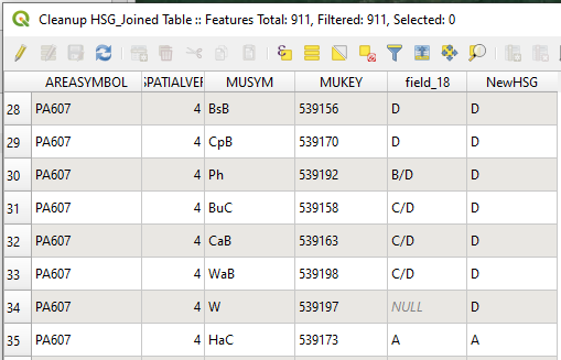
The first thing to do is to clean up the newly created HSG shapefile HSG_Joined Table.shp. In its field_18, there are features with value of Null (water area, for example) or A/D, B/D, C/D (for dual group definition, see this NRCS documentation), which are inherited from the original table muaggatt.txt. In order for the HSG shapefile (its raster file to be exact) to work properly with land cover raster file in the future, we will have to assign appropriate A/B/C/D to these features since there is no curve number provided for Null, or or A/D, B/D, C/D in Table 2-2 of the official NRCS TR-55 document. One way to do that is to assign D to all of them to be conservative (D has the least infiltration rate and thus bigger runoff potential).
- HSG_Joined Table.shp‘s field_18 can be manually edited to change Null, or or A/D, B/D, C/D to D as discussed above (Open Attribute Table and Toggle Editing Mode); Or if there are too many features (rows), it is easy to do it automatically by using Join attributes by field value. Create a simple CSV txt file which defines how to convert Null, or or A/D, B/D, C/D to D (Figure 14). Refer to the Step 9 above on Join attributes by field value.
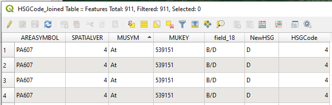
- Now let’s add another field (Integer Number) to the cleaned up HSG shapefile by applying the following relationship (A–>1, B–>2, C–>3, and D–>4). This can be done manually under editing mode; or you can utilize Join attributes by field value again by join it with a new CSV txt file (A,1;B,2;C,3;D,4). The result is shown on Figure 15. The purpose of convert HSG Group (A, B, C, D) to HSG Code (1, 2, 3, 4) is to create a raster file for future calculation, just like NLCD raster file using integer numbers to represent land cover types.
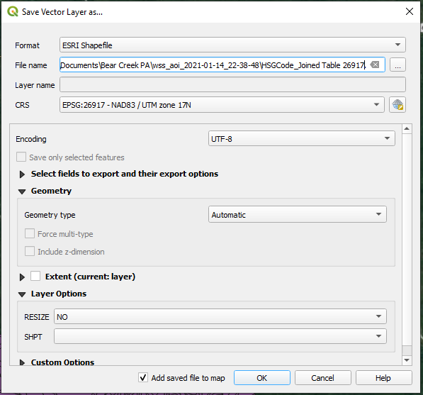
- It should be noted that the downloaded SSURGO raw data including shapefiles from Web Soil Survey is in reference to EPSG 4326. Before rasterizing it, now it is a good time to re-project the newly created shapefiles to a projected coordinate system (EPSG 26917 UTM Zone 17N for the example) which will also be used for the future H&H modeling projects. It is easy to re-project a shapefile: right click it and select Export–>Save Features As…, and then choose the desired projected coordinate system – CRS (Figure 16).
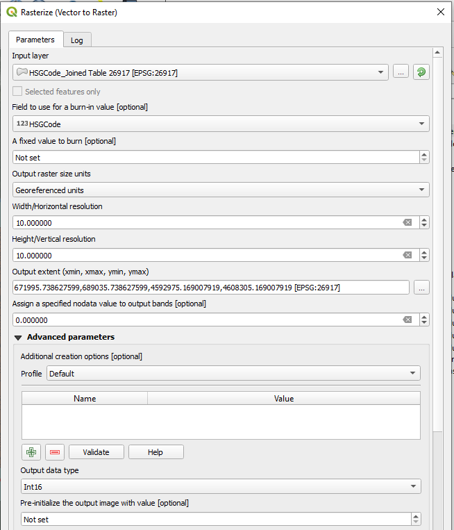
- Open a new QGIS project session and load the re-projected shapefile with HSG Code (1, 2, 3, and 4). Click top menu of Raster and choose Conversion–>Rasterize (Vector to Raster) to rasterize the shapefile. Field to use for a burn-in value [optional] is set as HSGCode; Select Not set for A fixed value to burn [optional], and the output raster size units is Georeferenced units with resolution number of 10, the same value as the land cover raster file created in Post 1 of 3 (10meter in this example since the UTM Zone 17N unit is meter). For the Output extent, choose the option of Use Layer Extent… and select the reclassified land cover raster file created in Post 1 of 3 as output extent – it is very important that the HSG raster file has the same extent and same resolution value as the reclassified land cover raster file so that the two files can work together to create a Curve Number raster file in Post 3 of 3.
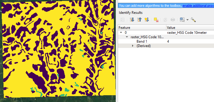
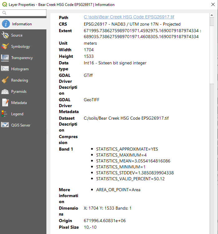
- Check the newly created HSG raster file (Figure 18). Per Figure 19, it is confirmed that raster file is created correctly as intended, with EPSG 26917 as CRS and Meter as Unit. The Pixel Size is 10 meter as defined at Step 4.
Some example files used in the demonstration for downloading:
- soilmu_a_aoi.shp (zip file, EPSG 4326)
- muaggatt.txt
- Soil HSG Code Shapefile before re-projection (zip file, EPSG 4326)
- Soil HSG code shapefile (zip file, EPSG 26917, UTM Zone 17N)
- Reclassified land cover raster file (EPSG 26917, UTM Zone 17N)
- Soil HSG code raster file (EPSG 26917, UTM Zone 17N)
- A sample soil report PDF file
Leave a Reply