Watershed Delineation Using SAGA Tools in QGIS

Update 1: SAGA tools used to be installed automatically with QGIS, but starting from QGIS version 3.3x around the year of 2022, QGIS dropped SATA package from its installation completely. Now to use SAGA tools, QGIS users are encouraged to work with third party plugins – one of them is Processing Saga NextGen Provider.

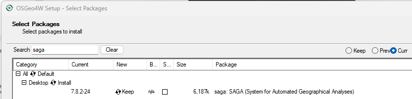
To make Processing Saga NextGen Provider work, the SAGA tool package first needs to be installed separately through OSGeo4W Setup (Figure A) since it is not part of QGIS installation any more.

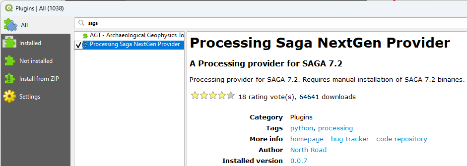
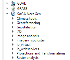
Next, search and install Processing Saga NextGen Provider plugin (Figure B). The SATA Next Gen icon should show up now in Processing Toolbox window (Figure C).

Update 2: in the new QGIS version 3.3X, the SAGA Upslope Area tool used for watershed delineation in this instruction may not work properly (discussions on Github). An easy way to circumvent the issue is to revise the Upslope Area tool’s description file – ta_hydrology_upslope_area.txt. This file usually is located in the Users\AppData folder (Figure D).

Locate and open the file and revise it by adding “|4” (pipe and number four) at the end of the first line of Upslope Area (no space in between) as shown in Figure E. Close and save it back, and now the Upslope Area tool should work in QGIS 3.3X.

Original Post before the above updates:

SAGA Tools are installed automatically with the installation of QGIS. Similar to watershed delineation using TauDEM Plugin or using Whitebox Tools Plugin, tools in SAGA can also be utilized to delineated a watershed.

To delineate a watershed upstream of an outlet (point of analysis), several steps are generally required:

1. Acquire a DEM of the area of interest and re-project it to a projected coordinate system, if it is in a geographic coordinate system originally;
2. Remove pit/fill sink;
3. Calculate flow direction;
4. Calculate flow accumulation and stream network;
5. Specify an outlet location which is the point of analysis;
6. Delineate watershed upstream of the outlet specified.

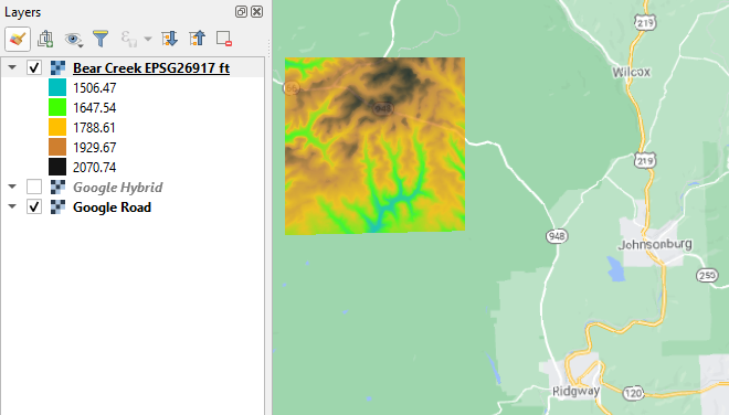
This post illustrates the watershed delineation method step by step using SAGA tools in QGIS. This demonstration is for Bear Creek watershed, located at about 9 miles west of Johnsonburg, PA (Figure 1). DEM is downloaded from USGS (https://viewer.nationalmap.gov/basic/#/) and a step by step instruction of downloading USGS DEM can be found in this post. USGS DEM’s CRS is in EPSG 4269 with elevation unit in meter. Prior to commencing watershed delineation, the USGS DEM was re-projected to UTM Zone 17N (EPSG 26917, NAD83) and clipped to an area just bigger than supposed watershed to reduce DEM file size. The DEM elevation was converted to foot using QGIS raster calculator.

Some of the files used for this demonstration can be downloaded by clicking this link which includes the re-projected DEM file Bear Creek EPSG26917 ft.tif, outlet shapefile, strahler raster file (stream network), the final delineated watershed shapefile.

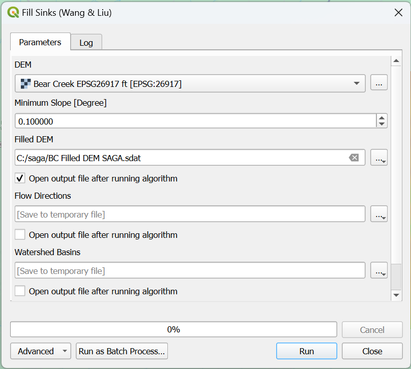
1. Fill Sinks (Wang & Liu) (Figure 2): In this example, the input file of is the re-projected DEM downloaded from USGS – Bear Creek EPSG26917 ft.tif and the output file is a new hydraulically connected filled DEM. In Fill Sinks (Wang & Liu), set the Minimum Slope as 0.01 (default value). Uncheck the options of Flow Directions and Watershed Basins since these two files are not needed at this step.

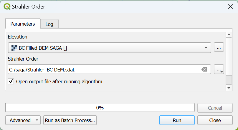
2. Run Strahler Order (Figure 3) using the filled DEM as input for Elevation.

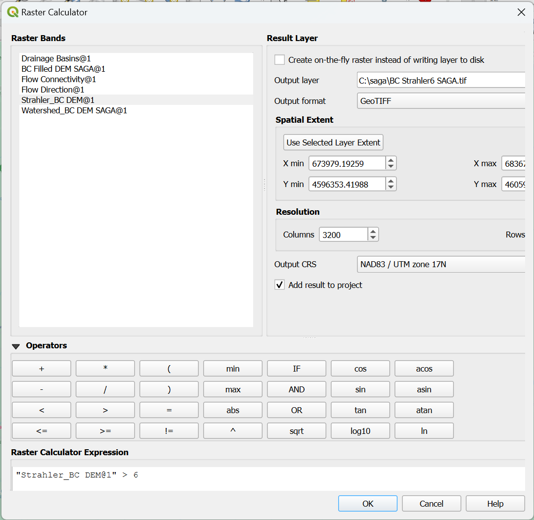
3. Use raster calculator to extract stream network (Figure 4). In this demo, an expression of strahler order >6 (equivalent to expression of strahler order >=7) is used. The threshold number 6 here is determined by trial & error. A smaller threshold will create a denser stream network and usually, 6, 7 or 8 is a good start number to try different threshold values to extract stream network.

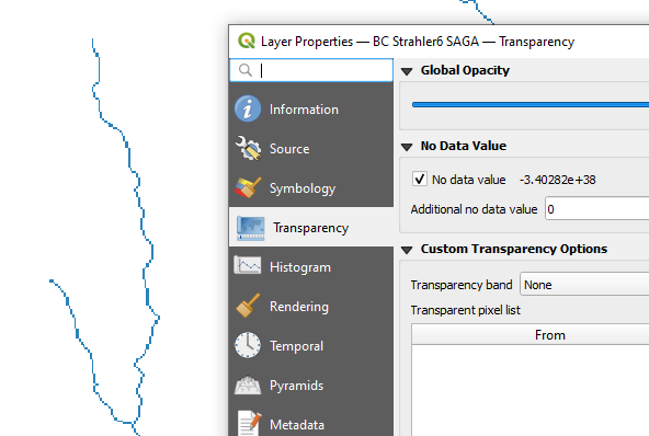
4. The product of Step# 3 is a new raster file of stream networks which uses pixels with value=1 for stream center lines. To highlight and display the stream center lines, turn off all pixels whose values are 0 by typing in zero (o) for Additional no data value in Properties—>Transparency (Figure 5).

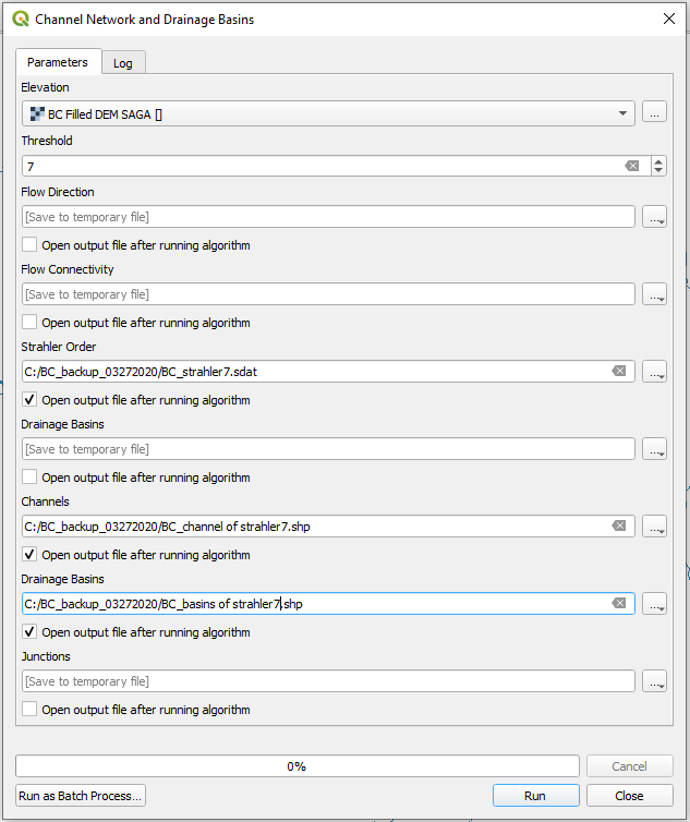
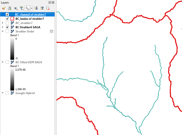
5. There is another SAGA tool – Channel Network and Drainage Basins (Figure 6) to create a stream network by using a strahler number as a threshold. The products of this tool are a stream centerline shapefile and a basin shapefile along with other raster files or shapefiles of your choice (Figure 7). The input raster file for Channel Network and Drainage Basins is the filled DEM and the stream center line definition threshold is set as 7 in this example (to match Step#3 raster calculator expression of strahler order > 6).

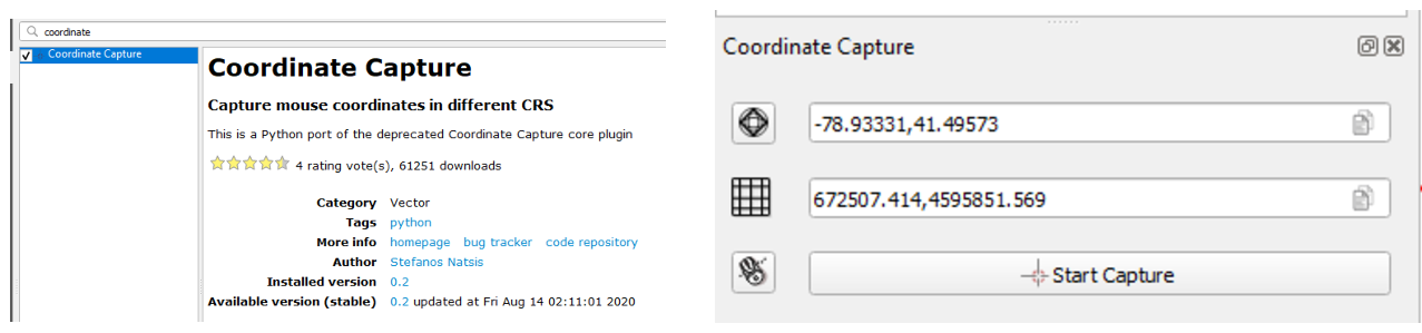
6. Determine the X/Y coordinates of the outlet point. One way is to zoom in to the stream network created at Step# 3 or Step# 5 and hover the mouse over the stream center line at your desired location to read the X/Y coordinates shown on the QGIS status bar at the bottom of the window or use Coordinate Capture Plugin to acquire the outlet point’s X/Y coordinate (Figure 8A).

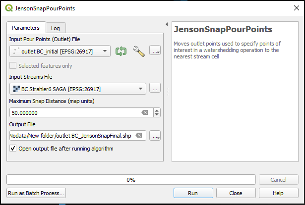
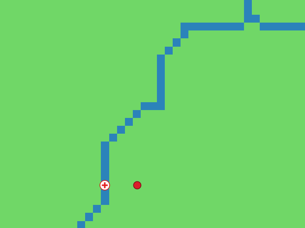
• Another method to determine the X/Y coordinates of the outlet point is to first create a point shapefile as the approximate outlet location and then use JensonSnapPourPoints of Whitebox Tools (WBT) Plugin to snap the point to the stream pixels (Figure 8B). In JensonSnapPourPoints, Input Pour Points (Outlet) File is the initial approximate outlet location shapefile and the Input Streams File is the stream network extracted at Step 3. As shown on Figure 9, the outlet point is moved to the stream center lines – blue pixels. Refer to this post to add X/Y coordinates as attributes to the point shapefile created by JensonSnapPourPoints.

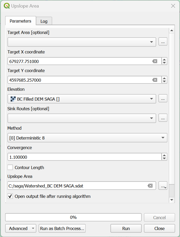
7. Use Upslope Area of SAGA to generate a watershed raster file (Figure 10). In Upslope Area, X and Y coordinates are used to define the outlet point, Method is Deterministic 8, Elevation file is the filled DEM, Convergence is set to 1.10, and leave Target Area and Sink Routes blank.

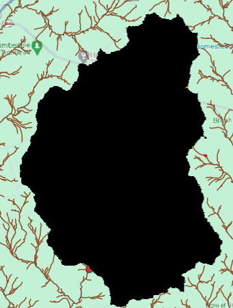
8. The raster watershed file (Upslope Area) created at Step# 7 is shown in Figure 11. In this raster file, the pixels within the watershed boundary have a value of 100 (white color) and the area outside the watershed (black color) has a pixel value of zero.

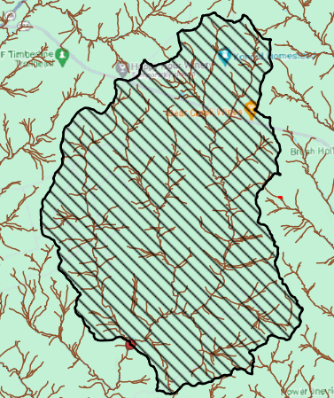
9. The raster watershed file can be vectorized (Figure 12) and then in the vectorized shapefile, delete the areas outside the watershed (Figure 13).

To calculate the longest flow path of the delineated watershed, the LongestFlowPath tool of Whitebox Tools (WBT) plugin can be utilized (Figure 14): the Input DEM File is the filled DEM and the Basins File is the raster watershed file (Upslope Area) at Step# 7.

In the shapefile created by LongestFlowPath, select the longest flow path line within the watershed and open its attribute table (Figure 15) to read its elevations, length, and slope. Ignore the lines outside of the watershed: these lines are created as a result of the raster watershed file including pixels=0 for the areas outside watershed.