Watershed Delineation Using TauDEM Toolbox in ArcGIS

TauDEM, developed by Utah State University is a set of tools to extract and analyze hydrologic information from topography as represented by a DEM. TauDEM is a set of standalone command line executable programs, but can also be installed in ArcGIS as a toolbox or in QGIS as a Plugin for easy application. Other hydrologic modeling and GIS tools, such as HEC-HMS and ACPF Toolbox, use TauDEM as GIS processing engine at back end.

TauDEM Plugin for QGIS introduced in this post does not work as of October 2022 since the author took down the repository website. Alternatively, TauDEM can be installed as an ArcGIS Toolbox as explained below.

1. Download TauDEM at its official website (Version 5.3.7 as of October 2022, TauDEM 5.3.7 Complete Windows installer). Run the executable file TauDEM537_setup.exe:
   • Click yes to the licensing agreements associated with the dependencies
   • When prompted to Choose Setup Type for GDAL, choose “Typical”
   • The following four (4) folders will be created automatically after installation:
     • a) C:\Program Files\Microsoft MPI\Bin\
     • b) C:\GDAL\
     • c) C:\Program Files\GDAL\
     • d) C:\Program Files\TauDEM\
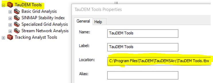
2. Open ArcMap ArcToolbox to add TauDEM Toolbox which is located at C:\Program Files\TauDEM\TauDEM5Arc\TauDEM Tools.tbx (Figure 1).

A DEM for Bear Creek watershed (9 miles west of Johnsonburg, PA) was downloaded from USGS National Map Website for watershed delineation. The files used for this demonstration can be downloaded here including the re-projected DEM file Bear Creek EPSG26917 ft.tif, outlet shapefile, the final delineated watershed shapefile, and Bear Creek watershed shapefile of HUC12 050100050603.

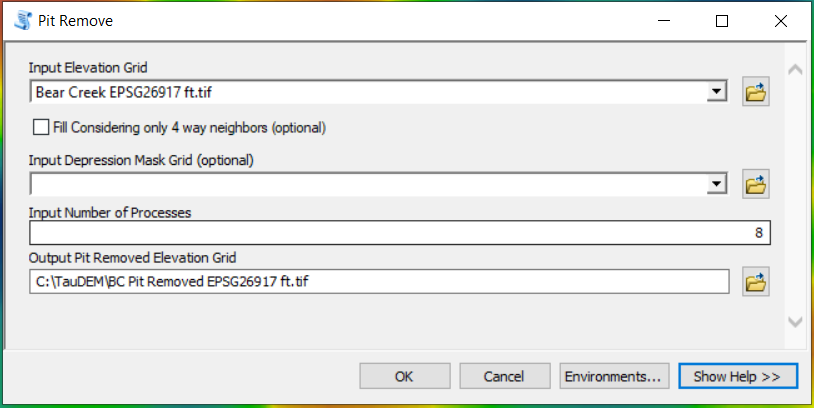
1. Pit remove (Figure 2): the input file is the re-projected DEM file – Bear Creek EPSG26917 ft.tif and the output file is a new hydraulically connected DEM – BC Pit Removed EPSG26917 ft.tif.

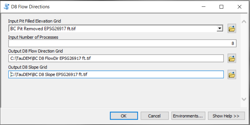
2. Run D8 Flow Directions (Figure 3): the input file is the new hydraulically connected DEM – BC Pit Removed EPSG26917 ft.tif and the output files are D8 Flow Directions file – BC D8 FlowDir EPSG26917 ft.tif and D8 Slope file – BC D8 Slope EPSG26917 ft.tif.

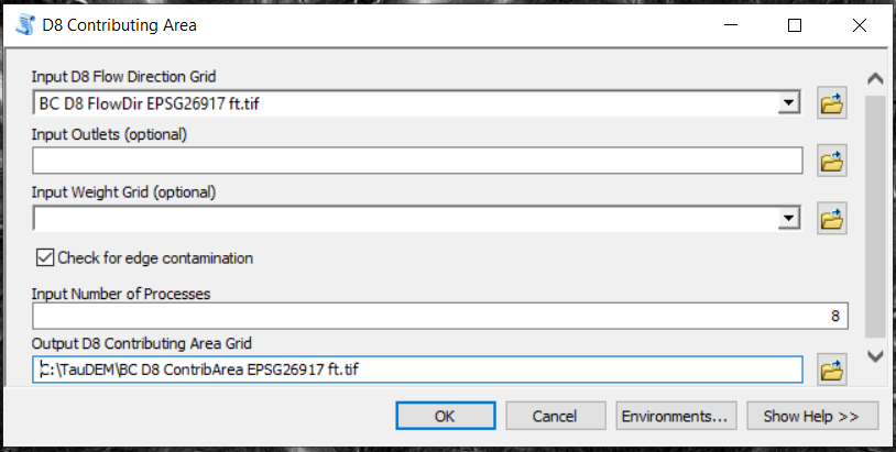
3. Run D8 Contributing Area (Figure 4): the input file is the D8 Flow Directions file – BC D8 FlowDir EPSG26917 ft.tif and the output file is BC D8 ContribArea EPSG26917 ft.tif. At this step, Outlets [optional] is left as blank and it is recommended to check on “Check for edge contamination“.

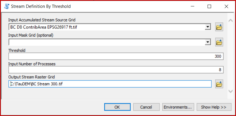
4. Run Stream Definition by Threshold (Figure 5): the input file (Input Accumulated Stream Source Grid) is the D8 Contributing Area file – BC D8 ContribArea EPSG26917 ft.tif and the output file is BC Stream 300.tif. At this step, Mask grid [optional] is left as blank and the threshold value is settled at 300 after trial & error. A smaller threshold value will result in a denser stream network.

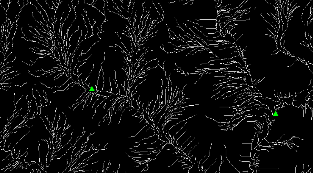
5. Create a point shapefile with two points as the outlet locations (the green triangular points in Figure 6). The outlet location will be your point of analysis. Ideally these points should be located on the stream network defined at Step 4 (white pixels in Figure 6), however it is difficult or sometimes impossible to put them on stream network at first attempt. This is acceptable: in this example, the two green triangular outlets are located close to the stream line pixels. At next step, they will be relocated to the stream line pixels using Move Outlets to Streams of TauDEM.

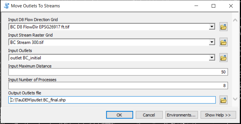
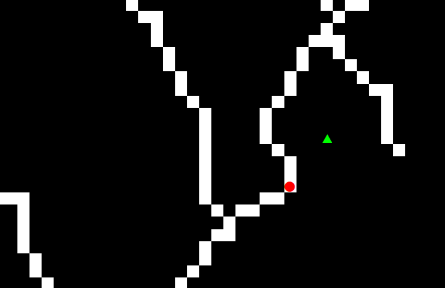
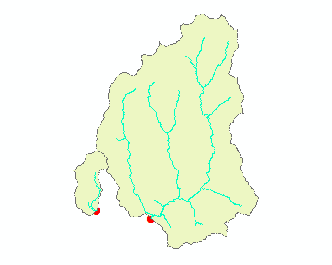
6. Run Move Outlets to Streams (Figure 7 and Figure 8): Input files are D8 flow directions file from Step 2, Stream raster file from Step 4, and initial outlet point shape file from Step 5. The output file is the relocated outlet point shapefile of outlet BC_final.shp. As shown in Figure 8, the relocated outlet (red circular point) is located exactly on the stream line pixels.

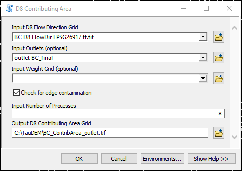
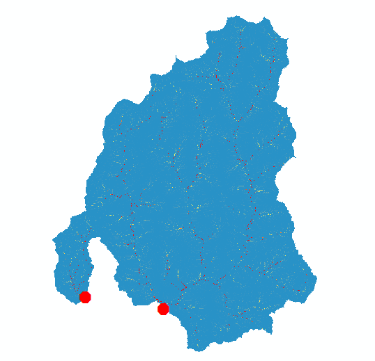
7. Run D8 Contributing Area gain (Figure 9): After the final outlet point shapefile is created at Step 6, run D8 Contributing Area again to delineate the watershed (upstream area) of the outlet. Different from Step 3, here Outlets [optional] is selected as outlet BC_final.shp from Step 6. It is recommended to check on “Check for edge contamination”. The output file is BC_ContribArea_outlet.tif, the contributing area for the watershed upstream of the outlets (Figure 10).

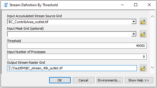
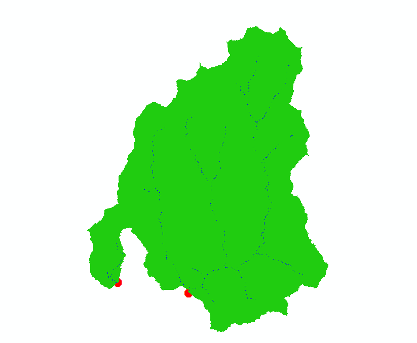
8. Run Stream Definition by Threshold (Figure 11) again: the input file (Input Accumulated Stream Source Grid) is the D8 Contributing Area file from Step 7 – BC_ContribArea_outlet.tif and the output file is BC_stream_40k_outlet.tif. At this step, Mask grid [optional] is left as blank and the threshold value is 40000 (trial and error, too small a value will end up with too many small subbasins being delineated). The output is a raster stream network upstream of the outlets (Figure 12).

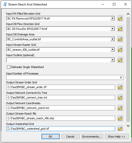
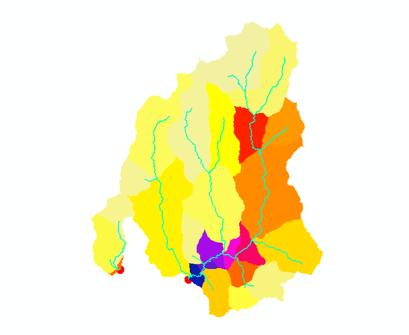
9. Run Stream Reach And Watershed (Figure 13): the input files are the pit removed/filled DEM, D8 flow direction raster file, D8 Contributing Area file from Step 7 – BC_ContribArea_outlet.tif, and raster stream network file from Step 8 – BC_stream_40k_outlet.tif. At this step, leave Input Outlets (optional) as blank. The output files include a watershed raster grid file and a stream reach vector shapefile (Figure 14).

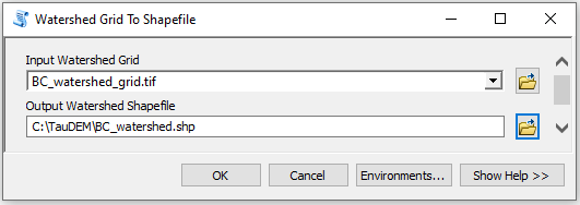
10. Run Watershed Grid to Shapefile (Figure 15): the input file is the watershed grid file from Step 9 and the output file is a shapefile (Figure 16).

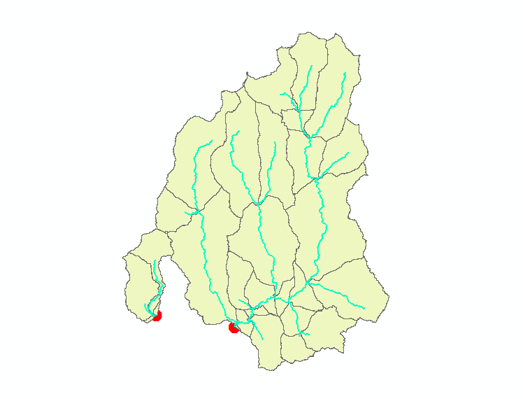
11. Optional: if desired, the subbasins in Figure 16 can be further dissolved/merged so there is only one combined subbasin/watershed for each outlet (Figure 17).