NOAA Atlas 14 Precipitation Depth (Annual Maximum & Partial Duration) and Temporal Distribution

NOAA Atlas 14 provides the latest official U.S. precipitation frequency (PF) estimates for various durations and frequencies with lower and upper bounds of the 90% confidence interval. PF estimates including point precipitation depth and intensity along with supplementary information (for example, temporal distribution) and documentation are available from the PF Data Server (PFDS).

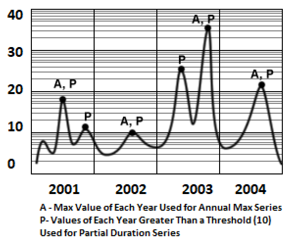
Atlas 14 provides two types of precipitation data – annual maximum and partial duration. Annual maximum only counts the largest event (A in Figure 1) of each year while partial duration includes all the events (P in Figure 1) greater than a threshold (10 in Figure 1). In Figure 1, for the year 2003, the P event on the left is ignored when calculating annual maximum since it is the second largest event in 2003, even though it is larger than the maximum event A in 2001, 2001, and 2004. For this reason, usually partial duration series generates greater values than annual maximum series of the same frequency (or AEP, annual exceedance probability). As the annual exceedance probability decreases (less frequent than 10-year event), the difference between annual maximum and partial duration data becomes negligible. Some agencies such TxDOT require using annual maximum precipitation data for most analyses and other agencies may prefer partial duration data. HEC-HMS Frequency Storm option provides a way to convert partial duration precipitation data to annual maximum precipitation data (and vice versa) for 10% (10-year), 20% (5-year), and 50% (2-year) events.

NOAA Atlas 14 Vol 11 Version 2 covers the Great State Of Texas and it divides the entire state into 3 climate regions, namely Region 1, 2 and 3 from west to east (Figure 2). Austin, Dallas, and San Antonio are located in Region 2 while Houston is within Region 3.

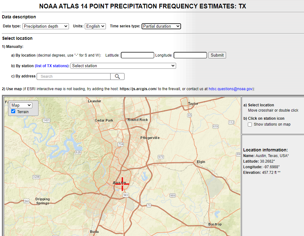
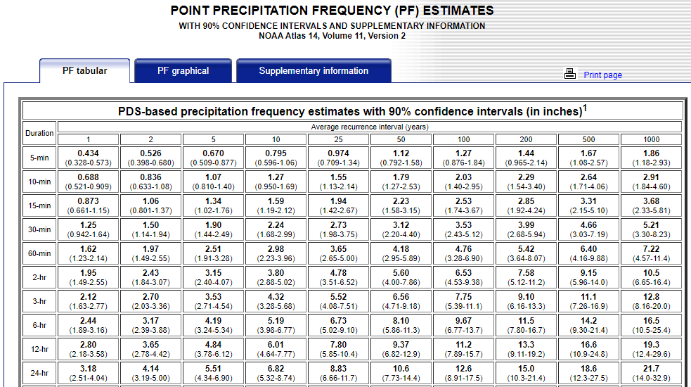
The following steps illustrate how to obtain point precipitation depth/frequency data and how to download and interpret the NOAA Atlas 14 temporal distribution by using Austin, Texas as an example area of interest. To get Austin’s point precipitation frequency data, visit NOAA PF Data Server (PFDS) website and click the map of Texas. In the next page (Figure 3), zoom in and double click the location of Austin, select time series type (Partial duration/Annual maximum) and data type (Precipitation depth/Precipitation Intensity, here intensity=depth/duration, for example, if 24-hr 100year precipitation depth is 12.6 inch, then its corresponding precipitation intensity is 12.6/24=0.525 inch/hr). The point precipitation frequency estimates and supplementary information are displayed below the location map on the same page (Table 1).

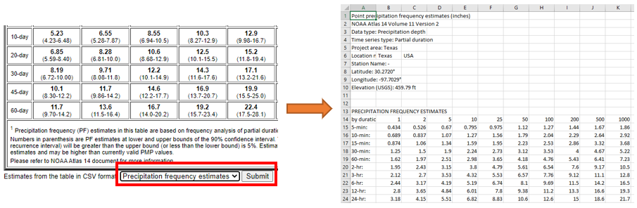
At the bottom of the table in Table 1, there is a link to download the entire table in CSV format (Figure 4) if desired.

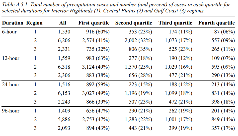
NOAA Atlas 14 temporal distributions are based on the historical storm events (cases) statistical analysis for each of the three climate regions of Texas (Figure 2). Table 2 lists the total number of precipitation cases being analyzed in Texas Region 1, 2, and 3 when developing Atlas 14 Vol 11 data. The total cases are further divided into four categories by the quartile in which the greatest percentage of the total precipitation occurred. For example, for Texas Region 2’s 24-hour data, totally 6153 cases were studied and among these 6153 case, 3027 (49%) cases have their greatest percentage of the total precipitation happen in the first 6 hours – first quartile of 24 hours.

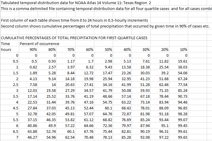
Temporal distributions of NOAA Atlas 14 are provided for 6-hour, 12-hour, 24-hour, and 96-hour durations. Click the Supplementary information Tab of Table 1 to download the time series of the temporal distributions (Figure 5). The temporal distributions for the duration are expressed as cumulative percentages of precipitation in probability terms. In addition to temporal distributions for all cases, separate temporal distributions are derived for four quartiles in which the greatest percentage of the total precipitation occurs (First Quartile, Second Quartile, Third Quartile, and Fourth Quartile). Hyetograph (cumulative rainfall distribution) can be developed based on the temporal distribution time series provided that the point precipitation depth is acquired following the steps above: select a percent of occurrence column in Figure 5 (90%, 80%, … 10%) you intend to apply, and then use the point precipitation depth to time the cumulative percentage to get the cumulative rainfall depth (unit: inch) at each time step. For a 24-hr duration rainfall event, at the end of its time series, since the time is 24 hours and the cumulative percentage is 100%, so the cumulative rainfall depth@24hr is the point precipitation depth acquired.

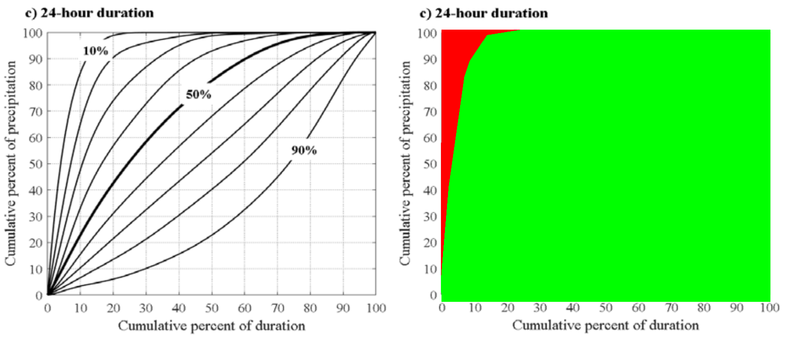
The temporal distribution curves represent averages of many cases and illustrate the temporal distribution patterns with 10% to 90% occurrence probabilities in 10% increments. For example, in Figure 6, the 10% curve indicates that 10% of the first-quartile precipitation cases have their distributions fall above and to the left of the curve (the red filled area of the right chart), while 90% of the first quartile precipitation cases have their distributions in the green filled area.

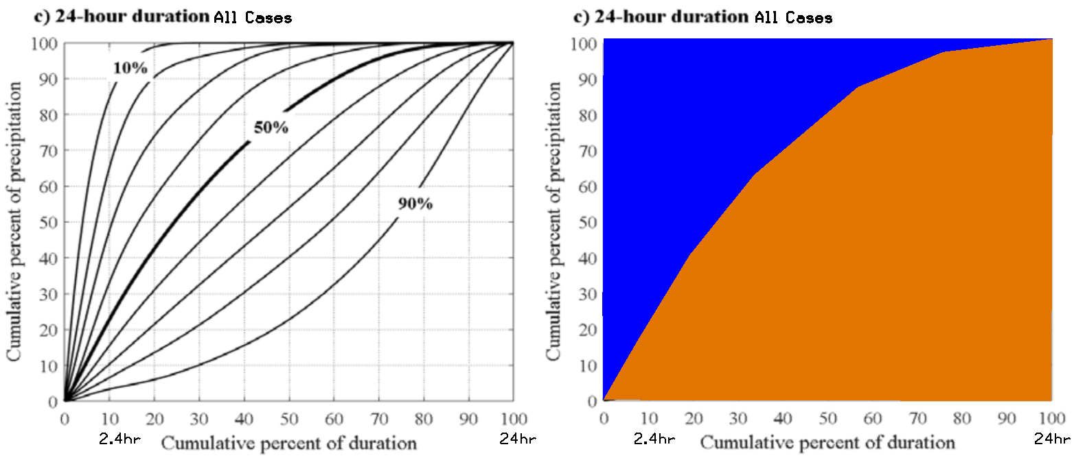
Another example of temporal distribution is shown in Figure 7, which represents the temporal distribution of 24-hr precipitation for all cases. In Figure 7, the 50% curve indicates that half (50%) of all precipitation cases have their distributions fall above and to the left of the curve (the blue filled area of the right chart), while the rest of 50% of all precipitation cases have their distributions in the brown filled area. Some studies use the 50% curve for rainfall distribution since the 50% curve is the median temporal distribution, while other studies calculate the corresponding runoff peak flows and hydrographs from all the 9 curves (10% to 90%) of a quartile and then pick up the percentage curve that provides the safest (the most conservative) design, which can be easily implemented by using the global storm function of XPSWMM. You may even apply multiple percent curves from different quartiles plus all cases to compare the results for the purpose of safe design.

For how to apply NOAA Atlas 14 temporal distributions in HEC-HMS as a hypothetical storm, refer to this post.

The above NOAA Atlas 14 temporal distributions shall NOT be confused with the NRCS rainfall distributions which are based on NOAA Atlas 14 precipitation depth data:

• NOAA Atlas 14 temporal distribution: not a “nested” storm, created by historical storm event statistical analysis for each climate region, and then grouped by different durations (6-hr, 12-hr, 24-hr and 96-hr ), quartiles (1st, 2nd, 3rd, 4th, and all cases), and percent of occurrence (10%, 20%, … 90%).
• NRCS rainfall distribution based on NOAA Atlas 14 precipitation depth data: a “nested” synthetic storm distribution, usually the storm duration is 24 hours, created by embedding shorter duration precipitation depths into 24-hr distribution. These new NRCS distributions are to replace the obsolete NRCS/SCS Type I, IA, II, and III distributions.

Refer to this post for more discussions on NRCS rainfall distributions.

Finally, which NOAA Atlas 14 temporal distributions should be used for a specific project? For a specific region and storm duration, there are 5 (1st, 2nd, 3rd, 4th quartiles plus All Cases) x 9 (10% to 90% 9 curves) =45 temporal distributions, and which one to choose? This question is hard to answer but here are some thoughts which might be helpful:

• First of all, always consult with the clients and regulating agencies for their input and agreement on if NOAA Atlas 14 temporal distributions are allowed and how to apply them.
• If a client gives green light on NOAA Atlas 14 temporal distributions but has no preference on how to implement them, you may be able to run the models with the 9 distributions of All Cases and pick the one resulting in the most conservative design.
• Or similarly, you could run the models with the 9 distributions of the quartile with the most cases and pick the one resulting in the most conservative design. For example: the 1st quartile almost always has the most cases in Table 2 for Texas and therefore use the 9 curves of the 1st quartile for a project in Texas.
• Run the models with the five 50% curves (1st, 2nd, 3rd, 4th quartiles plus All Cases) and pick the one resulting in the most conservative design. The 50% curves represent the average conditions.
• Of course, if budget and schedule permit, you can always run the models using all the 45 distributions and pick the one resulting in the most conservative design.