“Nested” Frequency Storms in HEC-HMS with Different Durations

In hydrologic modeling, “nested” storm distributions are widely used such as SCS Type I, IA, II, III, or the frequency storm in HEC-HMS. One of the advantages of a “nested” storm distribution is its capability to have shorter storm durations embedded inside a longer storm duration and thus a system’s hydrologic performances under different storm durations can be examined by a single model run using this longer storm duration. For more information about how to generate a “nested” storm distribution using the Alternating Block Method, refer to this post.

To test if a watershed’s peak flow varies with a “nested” storm’s duration or not, a simple HEC-HMS model was established using a 1.0 square mile subbasin. The 100-yr frequency storms with different durations were set up in the meteorologic model. Clark Unity Hydrograph was selected as the transform method with TOC=1.0 hr and R=2.0hr. Four scenarios were analyzed using different loss methods:

• 1. No loss method.
• 2. Deficit and Constant loss method
• 3. Green and Ampt loss method
• 4. SCS Curve Number loss method

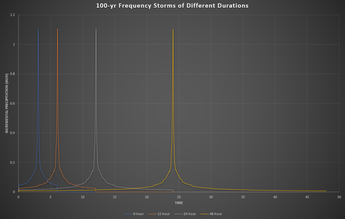
As shown in Figure 2, 4 frequency storms were created with durations varying from 6hr to 48hr. These frequency storms share the same precipitation depths of 5 min, 15min, 1hr,…, up to each storm’s duration.

Scenario #1: No loss method. This scenario is used to exclude any potential loss method impact to the peak flow values modeled in HEC-HMS. According to the results in Table 1, the peak flows of different frequency storm durations are almost the same, particularly for the two values under 24-hr and 48-hr storms. It is believed that the difference between the 6-hr/12-hr storm peak flows and the 24-hr/48-hr storm peak flows are due to the fact that the hyetographs of the shorter storm durations like 6-hr or 12-hr are not a “complete” one comparing to the longer duration storm hyetographs.

Scenario #2: Deficit and Constant loss method (Initial deficit=0.3 inch, maximum deficit=0.4 inch and constant rate=0.07 inch/hr). According to the results in Table 2, the peak flows of different frequency storm durations are almost the same, particularly for the two values under 24-hr and 48-hr storms.

For shorter duration storms like the 6-hour and 12-hour ones, the initial infiltration process to saturate soil has a much greater impact on runoff peak calculation than for longer duration storms, which is why the 6-hr and 12-hr peak flows are less than those of 24-hr and 48-hr. After the soil becomes saturated, as its name suggests, the infiltration rate is constant at 0.07in/hr up to each storm’s duration – this is the reason that the peak flows of 24-hr and 48-hr are identical.

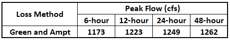
Scenario #3: Green and Ampt loss method (Initial Content = 0.05, Saturated Content =0.4, Suction = 3 inch, Conductivity = 0.1 inch/hr). According to the results in Table 3, the peak flows of different frequency storm durations are NOT the same, neither do they converge to a single value like Scenario #1 and #2, even though the difference is less than 10% between 48-hr and 6-hr storms ([1262-1173]/1173=7.6%).

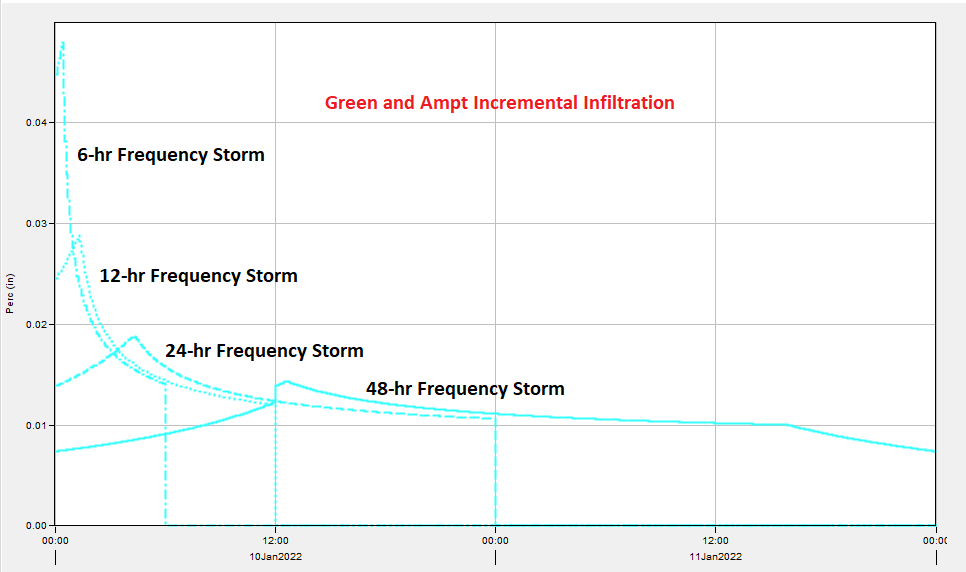
The infiltration behavior of Green and Ampt is different from Deficit and Constant loss method as shown in Figure 4 under different storm durations. The Green and Ampt infiltration loss rate never reaches a constant value and actually it is highly correlated to storm durations, which can explain why the peak flows do not converge under Green and Ampt loss method with different storm durations.

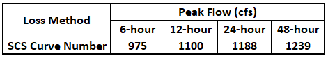
Scenario #4: SCS Curve Number loss method (Curve Number = 80). According to the results in Table 4, the peak flows of different frequency storm durations are NOT the same, neither do they converge to a single value like Scenario #1 and #2. The difference is 27% between 48-hr and 6-hr storms ([1239-975]/975=27%).

The infiltration behavior of SCS Curve Number is different from Deficit and Constant loss method as shown in Figure 5 under different storm durations. The SCS Curve Number infiltration loss rate never reaches a constant value and actually it is highly correlated to storm durations, which can explain why the peak flows do not converge under SCS Curve Number loss method with different storm durations.

Some thoughts on applying frequency storms in HEC-HMS models:

1. Using shorter duration frequency storms (6-hr, 12-hr) probably should be avoided, and instead, use 24-hr or longer duration ones since these longer duration storms have a more “complete” hyetograph and a system’s performance under shorter duration storms can be examined in a single model run using 24-hr, 48-hr, or even longer duration frequency storms;
2. Unlike peak flows calculated using Deficit and Constant loss method, the peak flow values under Green and Ampt or SCS Curve Number loss method will not converge with varying durations of a frequency storm and therefore caution should be taken when using Green and Ampt or SCS Curve Number loss method concurrently with frequency storms in HEC-HMS, especially if you want to use a single model run to evaluate a system’s performance under different storm durations.
3. Green and Ampt loss method results in a set of more consistent peak flow values under different frequency storm durations than SCS Curve Number loss method, and relatively speaking, it is a better choice (still not as good as Deficit and Constant loss method) for working with frequency storms in HEC-HMS.