Tailwater Boundary Condition in Storm Sewer Network Modeling

A storm sewer network discharges to a receiving waterbody through the outfall pipe and the receiving waterbody can be a river, channel, lake, ocean, or another storm sewer network (Figure 1). How to set up an appropriate tailwater condition is important for storm sewer network design and modeling. For drainage design, backwater HGL calculation requires a tailwater elevation at the outfall end of the system as a starting point, and for H&H modeling a tailwater elevation as boundary condition would impact the storm sewer network performance.

Generally, two types of outfalls – free outfall or non-free outfall – can be found in a storm sewer network and correspondingly, different tailwater conditions can be applied to them.

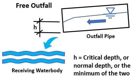
• Free outfall

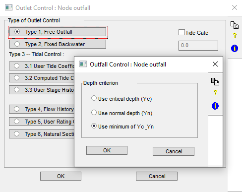
The receiving waterbody is so low that the outfall pipe will discharge to it “freely” (Figure 2) during the period of simulation. In other words, the receiving waterbody is NOT hydraulically connected with the outfall pipe. To run the model, the water depth in the free outfall node can be set as critical depth, normal depth, or the minimum of the two in XPSWMM (Figure 3A). In InfoWorks, an outfall node is treated as a free outfall by default and the water depth is always taken as the minimum of critical depth and normal depth, unless a level event is assigned to it.

Critical depth occurs when the flow in a box culvert or a pipe has a minimum specific energy and Froude Number is equal to 1.0. The critical depth is to be determined by the box culvert or pipe shape and flow rate when they meet the following relationship (Figure 3B): 

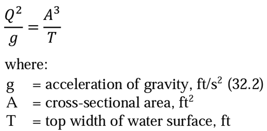
The critical depth can be solved directly for a box culvert or a rectangular shaped channel (Figure 3C).

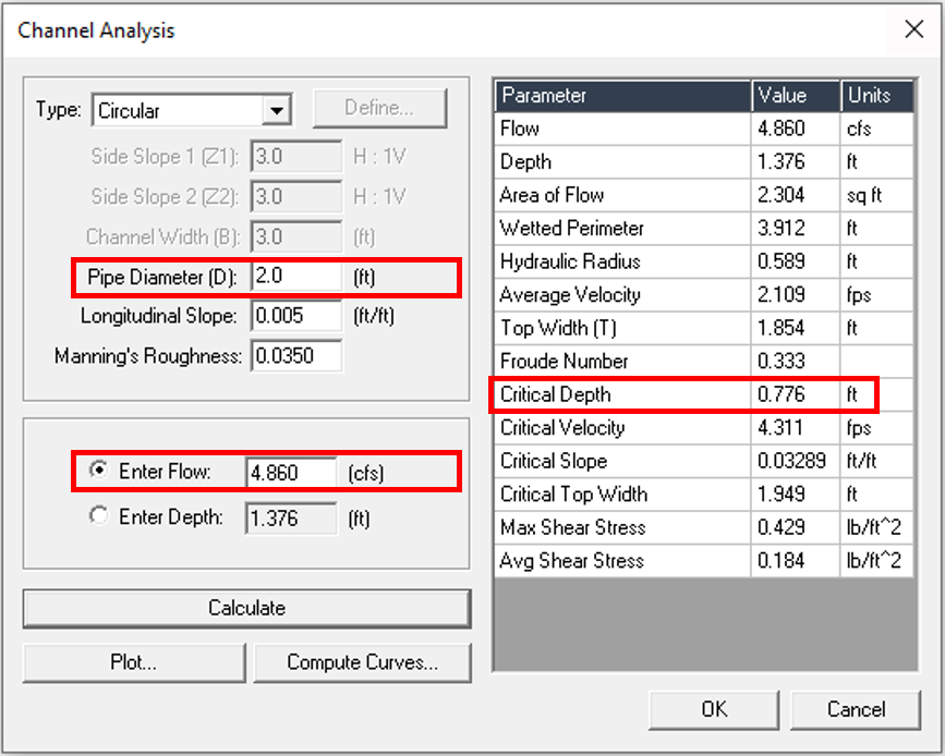
A trial and error procedure is usually needed to solve the equation in Figure 3B for circular pipes or other shaped channels. Hydraulic Toolbox can also be used to get critical depths for most common shaped pipes or channels (Figure 3D).

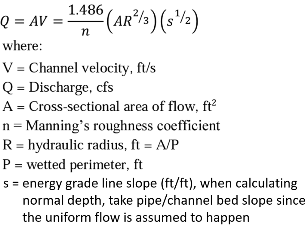
In addition to the flow rate and the pipe/box culvert shape, the normal depth also depends on the pipe slope and Manning’s n (Figure 3E). The Manning’s Equation can be easily solved in Hydraulic Toolbox (Figure 3F).

• Non-free outfall

The receiving waterbody and the outfall pipe is hydraulically connected and the receiving waterbody WSE (fixed or time-varying) impacts the storm sewer network performance by impeding flows through backwater (Figure 4).

There are several ways to evaluate and select appropriate tailwater elevations (WSE). A regulating agency’s drainage design manual often specifies what tailwater elevations should be used for storm sewer network HGL calculation under design level events such as 2-yr, 5-yr, or 10-yr, which can be borrowed as fixed tailwater elevations when modeling these frequent events. For example, City of Houston (COH) IDM requires using top of outfall pipe (if the outfall pipe is not submerged) as tailwater WSE for 2-year design event HGL calculation. FHWA HEC-22 states that for most designs the tailwater elevation can be taken as the crown (top) of the outfall pipe or can be a level between the top and critical depth of the outfall pipe.

Establishing a proper tailwater WSE at receiving waterbody may need to consider the discharge coincidental probability of two drainage basins: the usually larger drainage basin upstream of the receiving waterbody and the smaller storm sewer network basin. Because of the drainage area and time of concentration differences, the peak discharge from the storm sewer network will not arrive at the same time the drainage basin of the receiving waterbody peaks. For this reason, FHWA HEC-22 prepared a discharge coincidental occurrence table (Table 1) for 10- and 100-year design storms, which can be used to determine an appropriate tailwater WSE for storm sewer network design and modeling.

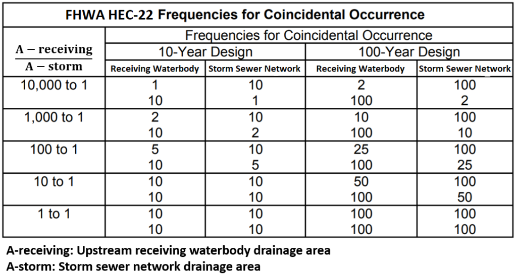
According to Table 1, if the drainage area of the receiving waterbody is 1000 square mile while the storm sewer network only has a drainage area of 1 square mile, the ratio of receiving area to storm area is 1000 to 1. When a 10-year design storm happens over the both basins, at the time the storm sewer network reaches its 10-year peak flow at the outfall location, the flow rate in the receiving waterbody is only the equivalent of a 2-year peak flow due to different TOC or peaking time. For a 100-year design storm, when the storm sewer network peaks, the corresponding flow rate/WSE at the receiving waterbody is only equal to a 10-year peak flow/WSE. As a matter of fact, COH IDM requires using 10-year WSE of the receiving waterbody for 100-year extreme event HGL analysis (or 2 feet below top of the bank) without explicitly mentioning the drainage area ratio assumption.

To determine WSE of the receiving waterbody under the required frequency events, a steady state HEC-RAS model may need to be established if solving Manning’s equation to get a normal depth is not sufficient.

In lieu of a fixed tailwater WSE, sometimes it is necessary or beneficial to use a time-varying tailwater WSE (stage hydrograph) as boundary conditions. Simulating a historical storm event is an example of requiring time-varying WSE which can come from receiving waterbody gage records. Another instance is when there is a need to do a detailed study on the impact of receiving waterbody WSE to the storm sewer network operation, particularly if the sizes (thus TOC) of the two basins are not too far off.

To determine time-varying WSE or stage hydrograph, an unsteady state HEC-RAS model of the receiving waterbody is needed. The inflow hydrographs used for the unsteady state HEC-RAS models must be coming from the same storm events to be used for storm sewer network modeling (Figure 5).

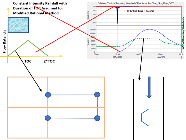
Some city or county governments allow storm sewer network modeling to use Modified Rational Method for inlet catchment runoff hydrographs and a common negligence is to use a receiving waterbody stage hydrograph (time-varying WSE) from other rainfall events as tailwater boundary conditions like what’s shown in Figure 6.

When selecting a tailwater elevation as boundary conditions, modelers may first want to refer to the criteria described on drainage design and H&H modeling manuals. Also, modelers are encouraged to study the H&H characteristics of the receiving waterbody and the storm sewer network and use a realistic tailwater elevation as the basis for modeling (be on the safe side but not overly conservative). It is always a sound engineering practice to establish or acquire an unsteady state HEC-RAS model for the receiving waterbody, and use time-varying tailwater WSE (stage hydrograph) from the same storm events for storm sewer network as boundary conditions.

If a community is subject to fluvial flooding from high tailwater of the receiving waterbody during extreme storm events, the local storm sewer network will be overwhelmed, and the community will be inundated during the high tailwater period. The only way to mitigate this type of flooding is to lower tailwater WSE by improving receiving waterbody conveyance and other measures such as diversion or detention. These measures normally require coordination between federal, state, and local government agencies for permitting and funding and take years to work things out. While waiting, the community, however, still can do its own part to model/design/upgrade the storm sewer infrastructures to reduce local flooding during frequent storm events such as 2-year, 5-year, or 10-year. For this type of modeling, the tailwater boundary condition should be selected carefully, and it should not be the high tailwater conditions which would cause fluvial flooding no matter what is proposed to the storm sewer network.