Gridded SCS Curve Number Loss Method and ModClark Transform Method in HEC-HMS

ModClark method is a distributed rainfall-runoff transform method available in HEC-HMS. To apply ModClark transform method, a basin (watershed) is subdivided into a gridded system and each grid cell is a small sub-watershed where hydrology calculation happens. A structured discretization method is required in HEC-HMS for ModClark method (refer to this post on how to set up structured discretization and this post for ModClark transform method introduction).

ModClark can work together with either a lumped loss method (for example, SCS Curve Number using basin average CN – refer to this post) or a gridded loss method which account for spatial variations of loss rates. ). To apply the gridded SCS Curve Number method in HEC-HMS, a curve number raster file has to be created first and then it needs to be imported into a HEC-DSS file as a gridded DSS record. An importing tool (Vortex Importer) developed by HEC can be downloaded here and the instruction is provided by HEC on how to import a curve number raster file to a DSS file.

It is worth emphasizing that the Curve Number grid needs to be created the same way as the basin is discretized in terms of the projection system and grid cell sizes. In the example below, the basin has the structured discretization set to SHG and 50 meters as the cell size and so the Curve Number grid also needs to be set to SHG with 50-meter x 50-meter grid cells. If using gridded precipitation, the precipitation grid projection must also be consistent with the Curve Number grid and basin discretization projections while the precipitation grid cell size can be different.

An example HEC-HMS project can be downloaded here and it includes two basins: Basin of PistolCreek is to use Gridded SCS Curve Number loss method while the other one (Basin of PistolCreek-Ave CN) will use the conventional SCS Curve Number Method (basin average CN=77.53).

Open the example HEC-HMS project and after importing the curve number raster file to a DSS file, a new SCS Curve Number grid data needs to be added (Figure 1).

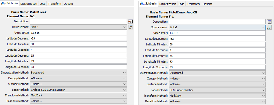
Change the example project Basin of PistolCreek loss method to Gridded SCS Curve Number and select the Curve Number grid data just added (Figure 2 and Figure 3). Make sure the other basin (Basin of PistolCreek-Ave CN) is using the conventional SCS Curve Number method for loss with CN=77.53 (Figure 2 and Figure 3). All other settings including precipitation are the same for the two basins.

The outflow hydrographs of the two basins are similar (Figure 4) and their peak flows are close too: Q-peak of ModClark-Gridded CN is 812.9 cfs while Q-peak of ModClark-Avg CN is 829.6 cfs.

Refer to this page at USACE HEC website for other grid type definition (Part C name in DSS pathname) and their default units.