Node Flooding and Ponding, Overland/Street Flow In 1D XPSWMM Modeling

Even if 2D modeling by XPSWMM, PCSWMM, HEC-RAS, and InfoWorks has become popular these days, 1D modeling still holds its ground on storm water management and flooding study due to several advantages over 2D:

1. Mainstream storm water modeling approach for the last half century and having a large user base in the engineering community
2. Less amount of data required to establish a 1D model and smaller model file sizes
3. Faster model run which means more time for model debugging, validation and calibration, and alternative study under a limited budget and a tight schedule
4. Capable of generating relatively reliable results when applying proper modeling skills and reasonable assumptions
5. Methodology and results widely acceptable by reviewing and regulating agencies

SWMM including EPA SWMM and the proprietary software XPSWMM/PCSWMM was originally developed to model 1D flow in a storm sewer network or an open channel system and extra considerations must be given when a 1D model is to deal with node overflowing or surface flooding. Different methodologies compute HGL in an overflowing node differently which in turn would impact 1D flow in a pipe or a channel.

For easy discussion purpose, flooding and ponding are defined as below:

Flooding: the storm sewer system is overwhelmed and the node overflows are lost from the system.

Ponding: the storm sewer system is overwhelmed but the node overflows are temporarily stored at a ponded area above the node spill crest or rim. The stored volume can be released back to the storm sewer system at a later time if the system capacity allows.

This post is to focus on 1D storm sewer network modeling in XPSWMM. When a storm sewer network is overwhelmed, any storm water exceeding its capacity will rise up in nodes until the water level reaches the ground surface (spill crest) and at this point XPSWMM has different ways to handle the situation:

1. Set up Spill Crest as the actual ground or top of node elevation while the Ponding is “None” (Figure 1). Any excessive water above node spill crest elevation will get lost from the system through nodes (no water loss through links in XPSWMM) – flooding happens. This option probably should be avoided at all costs since the lost water will not be accounted for by the model. The maximum HGL at a node is its spill crest under this setting.

2. Set up Spill Crest to an arbitrarily high value to prevent the water from getting lost while the Ponding is “None” (Figure 2). The extremely high Spill Crest will contain the water in the system (HGL can go up as high as Spill Crest), but it should only be used sparsely in a screening level study since it may result in unrealistically high HGL and flow rates in the storm sewer network. Only a few field situations can be modeled properly by this method such as the nodes at each end of a forcemain or a bolted or sealed manhole. No flooding or ponding happens in this scenario.

3. Similar to #2 above, sealing a node will also prevent water loss (Figure 3) in which HGL can go up as high as needed. A bolted manhole is an ideal candidate for applying the “Sealed” ponding option. No flooding or ponding happens in this scenario.

In a real world, if a storm sewer system is overwhelmed, the excessive water will spill over from the inlet or manhole openings and then ponds on the ground or flows downstream along an overland path such as street gutters. In 1D XPSWMM, this is modeled by allowing ponding, a storage node with depth measured from spill crest, a dual drainage system, or their combination.

4. Setting the ponding option as “Allowed” will allow excessive water to be kept temporarily in a ponding area above the overflowing node and only return to the subsurface storm sewer system at a later time (Figure 4). This is a quick way to account for surface flooding without causing an unrealistically high HGL and can be used for preliminary analysis. According to XPSWMM manual, the ponding area is calculated as A * exp (B * Ponding Depth), which can be further edited in Hydraulic Job Control/Junction Defaults. XPSWMM Manual suggests that A has a typical value of 1000 to 5000 and B usually ranges from 1.0 to 5.0. To model a constant ponding area, set B to an extremely small value like 0.00001.

5. For a more detailed study, use a storage node with its ponding option set as “Allowed” (Or “None“, the setting here does not matter) and its storage depth being measured from Spill Crest (Figure 5). This option works in a similar way to #4, with only the ponding area being user-defined to better describe the field situation. In the stepwise linear storage method window (Figure 6), the maximum defined depth probably should be greater than the expected ponding depth; otherwise, XPSWMM will re-use the last surface area by assuming a vertical wall surrounding it to calculate ponding depths above the maximum defined value.

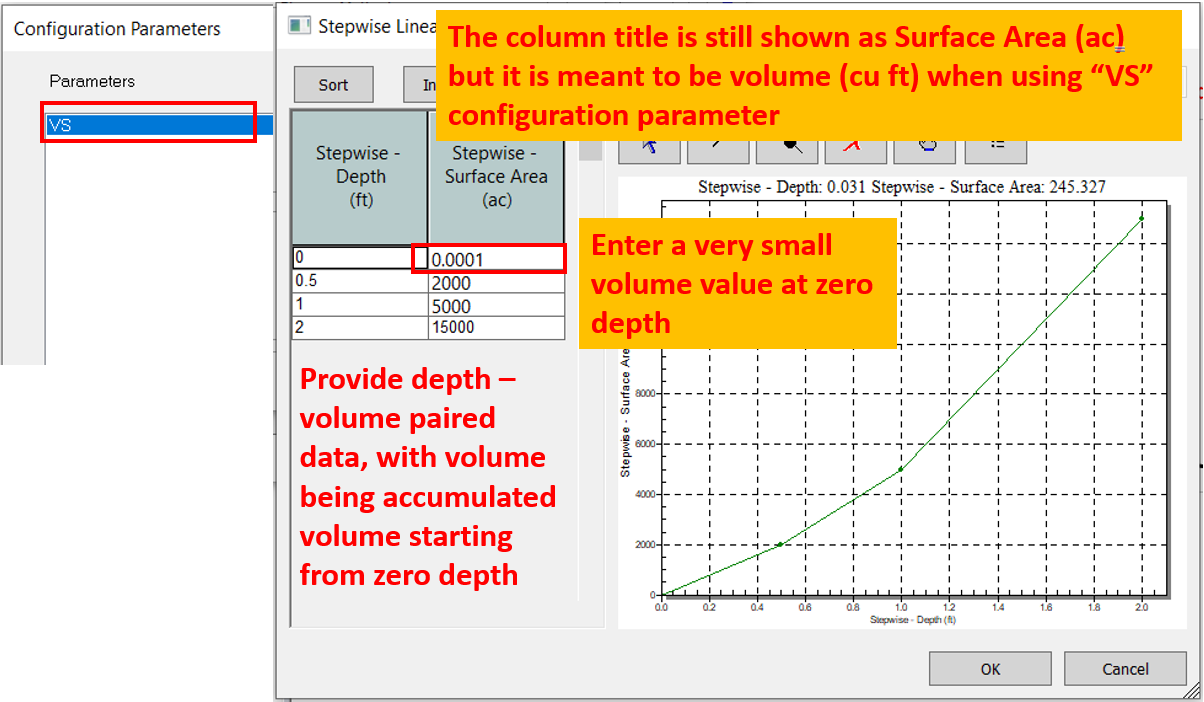
The default stepwise linear storage method requires a paired data set of depth and surface area, however, if desired, a modeler can override the program setting using “VS” configuration parameter to enter depth and volume values (Figure 7).

Using a storage node to model a ponding area above node spill crest can be applied to anywhere there is a node overflowing issue and the spilled water needs to be stored temporarily according to the local topography, although the most ideal locations may be at depressed areas such as a sag inlet or a low area with an inlet in the middle. To facilitate inter-storage area flow transfer, a weir can be set up at the high ground boundary of two neighboring storage areas (Figure 8).

6. The Multi Link option of XPSWMM can be used to model a dual drainage system (minor system – subsurface storm sewer network; major system – open channel flow in street/overland/ditch). Usually the node spill crest should be raised to match the highest elevation that the open channel cross section is representing. For example, if the major system is represented by a link using a natural section from road ROW to ROW, the node spill crest should be raised from its normal position by D as shown in Figure 9. Under some rare situations, the spill crest may need to be raised by more than D to contain higher than expected HGL and in this scenario two vertical glass walls will be assumed at each end of the open channel cross section to match spill crest (assuming VERT_WALLS=ON, refer to this post for more details).

A single link can be converted to a multi-link manually by right clicking the selected single link and choosing Multi Link as shown in Figure 10.

XPSWMM also has a tool to help convert a single link (pipe) to a dual drainage system if the major system is to be defined by a natural section shape. First select as many as single links that need to be converted, and then go to Tools —>Dual Drainage Batch Converter… to make the conversion (Figure 11).

In Figure 11, the max depth is usually left as 0 to let XPSWMM calculate the natural section shape depth as default (Figure 12). After conversion, the major drainage system conduit inverts are to be set at the original node spill crests, while the new node spill crests will be automatically increased by the calculated natural section shape maximum depths.

In a dual drainage system, the node’s inlet capacity feature can be turned on (Figure 13, this example uses Maximum Capacity – the simplest inlet capacity setting for demonstration purpose) to model an inlet’s restriction to incoming flow: only the flow not exceeding the inlet capacity will drop into the inlet chamber to be carried away by the subsurface storm sewer, while the remaining will flow down the major system – a street or an overland open channel.

Enabling a node’s inlet capacity will split the original node into two by XPSWMM internally: a “top” node (connecting major system) and a “bottom” subsurface node (connection minor system) which is denoted by “$I” (Figure 14 and Figure 15).

The two internal nodes are connected by a rating curve (Node name + “$R“) defined by the inlet capacity setting (Figure 16). The flow captured by the inlet capacity rating curve can be viewed in the result window (Figure 17).

When the inlet capacity feature is enabled in a XPSWMM model, extra attention should be paid to model stability. In this example, the maximum inlet capacity had to be lowered from 8 cfs to 4 cfs to get a stable captured flow result as shown in Figure 17.

If the inlet capacity is not enabled in a dual drainage system, an internal node with “$I” will not be created. In this case, a surface open channel will only receive inflows from the nodes it is connected to when the water levels in the nodes rise above the open channel invert.

The settings for ponding and sealed (bolted) options in PCSWMM or EPA SWMM are a little bit different from those in XPSWMM.

1. In PCSWMM or EPA SWMM, if a junction is sealed, a surcharge depth needs to be provided in this junction attribute table. Use an unrealistic big value to ensure the HGL can go as high as needed.

2. The ponded area is constant in PCSWMM or EPA SWMM which is entered in junction attribute table (Figure 18). If both ponding and surcharge are enabled and specified for a junction, the surcharge depth will be ignored.

3. If the ponded area needs to be modeled with a user-defined depth Vs. elevation relationship, this junction should be converted to a storage node. In Figure 19, a storage curve is defined to model a junction with a user-defined ponded area, in which the node depth is 8ft and the diameter is 4ft (so the area from 0 to 8ft is 12.57 sq ft).

PCSWMM can also add and model a dual drainage system. After a minor system is set up in PCSWMM, select the minor system conduits and go to Map Panel–>Tools–>Conduits–>Dual Drainage Creator to create a major system (Figure 20).

The newly created dual drainage system is shown in Figure 21, in which a separate set of junctions and conduits (street sections) are connected to the minor system through outlets for inlet control. The outlet rating curve type can be based on depth above outlet invert (inlet node invert + outlet’s inlet offset) or head difference between inlet and outlet nodes. Water can flow in either direction in an outlet depending on which node has a higher HGL. When the head at the inlet node or outlet node is lower than the outlet invert, the head option is the same as the depth option.

The outlet rating curves can be generated by referring to FHWA HEC-22 and the processes is even complicated for on-grade inlets. To avoid developing rating curves, the outlets shown on Figure 21 for inlet control purpose may be replaced by orifice links with a typical discharge coefficient of 0.60 to 0.65. A grate inlet may be modeled by a bottom orifice while a curb opening inlet can be approximated by a side orifice.

The ponding option in SWMM is a quick and easy way to keep excessive storm water in the system, however, it should NOT be used extensively. A node with ponding option probably should be in a sump/sag location, and for a on-grade inlet, enabling its ponding option does not make a lot of senses. It is tricky to estimate a ponded area: too small a ponded area will result in high HGL which may cause reverse flows; on the other hand, too big a ponded area may not be realistic (ponded area is NOT catchment area!). Several iterations may be needed to get a reasonable result in terms of ponded area, total ponded volume, and maximum ponded depth.