Land Cover Layer and Manning’s n in HEC-RAS 6.0

In HEC-RAS 6.0, users have the option to import either raster landcover files or vector landcover files to create a land cover layer which will then be used to associate manning’s n values with different land cover types for 2D domain modeling. National Land Cover Dataset (NLCD) is available for the entire lower 48 states of US (CONUS) and it provides good land cover data in raster format for HEC-2D modeling. The latest land cover dataset is NLCD 2016 which can be downloaded from https://www.mrlc.gov/viewer/. NOAA developed a nationally standardized land cover for the coastal areas of the U.S. through the Coastal Change Analysis Program (C-CAP). The latest 2016 C-CAP data in raster format can be downloaded from NOAA C-CAP website. 

HEC-RAS 2D domain Manning’s n values are defined by three levels of layers:

1. Land Cover Layer – this is the basis of Manning’s n. The Land Cover Layer is usually created by importing land cover dataset in raster format. You can also create a land cover layer by using vector files. Once a land cover layer is generated, Manning’s n values need to be assigned to different land cover types.
2. Classification Polygons under Land Cover Layer – polygons created by modelers to re-define areas that are not represented well by Land Cover Layer. Manning’s n established in the Classification Polygons will override Manning’s n defined in Land Cover Layer. For example, the NLCD dataset usually is not good enough for main channel modeling of a river and users are encouraged to create their own main channel classification polygons with appropriate Manning’s n value.
3. Calibration Regions – Manning’s n value can be further refined or overridden by using calibration regions (polygons).

This post is a step by step instruction on how to set up a land cover layer with appropriate Manning’s n value for HEC-RAS 2D using NLCD 2016 dataset. Before creating the land cover layer, set up a HEC-RAS 2D model with the required projection system, terrain layer, and 2D flow areas .

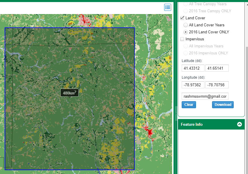
1. Go to https://www.mrlc.gov/viewer/ to download NLCD 2016 raster data for your project area. Select a rectangular box bigger than your project area to ensure that your project area is well covered. After providing your email and clicking Download Button in Figure 1, go to your email to click the link sent from MRLC@USGS.

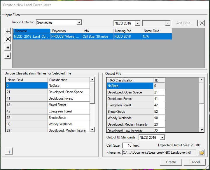
2. The downloaded NLCD raster file is in reference to EPSG 5070 – Albers Conical Equal Area Projection NAD 83 and can be imported into HEC-RAS 2D directly, letting HEC-RAS handle the re-projection if HEC-RAS projection system is different from the NLCD raster file (in the demo, the projection system is set as EPSG 26917, UTM Zone 17N, Unit: meter). To create a new Land Cover Layer using the downloaded NLCD 2016 raster, go to top menu Project, click Create a New RAS Layer… and then select Land Cover Layer (Figure 2). Import Extends can be set as Terrains, Geometries, or Entire Input File depending on your project needs. It should be noted that in Figure 2, the cell size is shown as 10 feet, but it is believed the unit of feet is a display error due to the bug of HEC-RAS 6.0 – the correct unit should be shown as meter since the demo project’s projection system EPSG 26917 has a unit of meter.

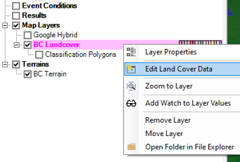
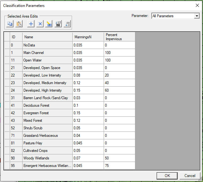
3. Right click the land cover layer just created (BC Landcover in magenta color in Figure 3) and select Edit Land Cover Data to type in Manning’s n values for each type of land cover. You can refer to this post for guideline of selecting Manning’s n for different land cover types. Percent Impervious data is only to be used when modeling 2D infiltration. Figure 4 shows the percent impervious for various land covers used in the BaldEagle example project coming with HEC-RAS 6.0 installation. No infiltration is to happen on impervious areas.

3A. If desired and needed for 2D infiltration loss modeling, a second land cover layer can be created to supply percent impervious values while let the first land cover layer created above to provide Manning’s n values only. Refer to this post for importing NLCD impervious raster files to create the second land cover layer.

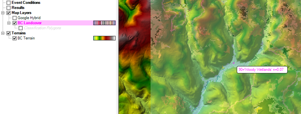
4. Make sure the land cover layer is checked on and highlighted in magenta color and hover mouse over map view, Manning’s n value will show up for the location your mouse stays at (Figure 5).  

5. Select and highlight Classification Polygons under Land Cover Layer, right click and select Edit Layer. In the editing mode, draw polygons to re-define areas where you want to override land cover layer Manning’s n values. Draw as many polygon areas as needed and provide name and Manning’s n for each polygon.
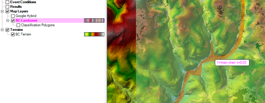
6. Select and highlight the land cover layer in magenta color and hover mouse over map view, Manning’s n value will show up for the location your mouse stays at (Figure 6). The Manning’s n value in Figure 6 is 0.03, different from Manning’s n value (0.07) in Figure 5 because at this location a classification polygon is created to override Manning’s n value.

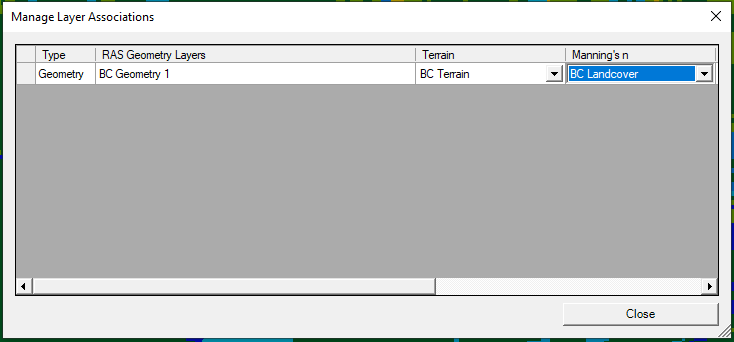
7. Go to top menu Project, click Manage Layer Associations… and then select Land Cover Layer just created under Manning’s n column for the geometry you are working on (Figure 7).

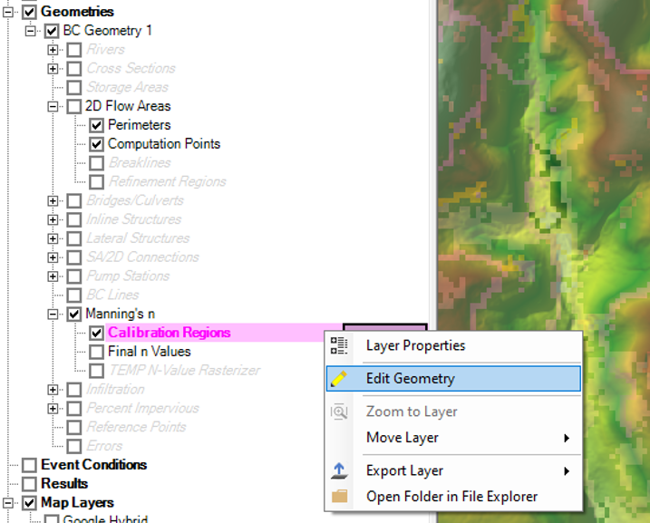
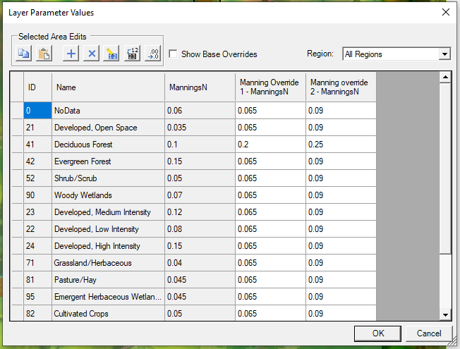
8. Now let’s further refine Manning’s n value by using Calibration Regions. Go to Geometries —> Manning’s n —> Calibration Regions, highlight it in magenta color, right click to select Edit Geometry (Figure 8). In the editing mode, draw polygons as calibration regions where you want to further re-fine Manning’s n values. Provide name and type in new Manning’s n value as shown in Figure 9. In Figure 9, two calibration regions are created and new Manning’s n values are provided (0.065 and 0.09 respectively except for Deciduous Forest – 0.2 and 0.25)

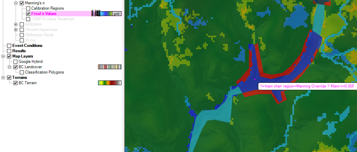
9. Select and highlight Final n Values under Manning’s n and hover mouse over map view, Manning’s n value will show up for the location your mouse stays at (Figure 10). The Manning’s n value in Figure 10 is 0.065 as defined in Step 8, different from Manning’s n value in Figure 5 or Figure 6 because at this location a Calibration Region is created to further override Manning’s n value defined in Land Cover Layer (Figure 5) and Classification Polygon (Figure 6).

Manning’s n values to be used in HEC-RAS 2D modeling are stored in Final n Values layer as explained in the steps above. It is worth noting that HEC-RAS 6.0 provided 3 types of layers to define Manning’s n values, however, only the land cover layer is required, and Classification Polygons and Calibration Regions are optional.